Adaptive vs Rational Expectations
Macroeconomics (M8674), March 2025
Vivaldo Mendes, ISCTE
vivaldo.mendes@iscte-iul.pt
1. Introduction
Why Models with Rational Expectations (RE)?
Economics is different: contrary to physics, biology, and other subjects, in economics most decisions are based on the agents’s expectations
Two competing views in economics to deal with the formulation of expectations:
- Backward-looking (or adaptive) expectations
- Forward looking (or rational) expectations
How relevant are they?
Let us look at some simple examples.
Example 1: the evolution of public debt
The evolution of public debt as a percentage of GDP \((d_t)\) is given by: \[d_{t}=p+\left(\frac{1+r}{1+g}\right) d_{t-1}\]
\(p\) is the primary deficit as a % of GDP, \(r\) is the real interest rate paid on public debt, and \(g\) is the growth rate of real GDP.
\(d_t\) is a pre-determined variable because is determined by observed past values.
The stability of \(d_t\) depends crucially on whether: \[r>g \quad , \quad r<g \quad , \quad r=g\]
In this equation, none of its elements depends on future expectations.
Example 2: a financial investment
Consider a financial asset:
- Bought today at price \(P_t\), and pays a dividend of \(D_t\) per period.
- Assume a close substitute asset (e.g., a bank deposit with interest) that yields a safe rate of return given by \(r\).
A risk neutral investor buys the asset if both returns have the same expected value: \[\frac{D_{t}+ \mathbb{E}_{t} P_{t+1}}{P_{t}}=1+r\]
Solve for \(P_t\), and to simplify define \(\phi = 1/(1 + r)\), to get \[P_{t}= \phi D_{t}+ \phi \mathbb{E}_{t} P_{t+1}\]
How do we solve such an equation? \(P_t\) is called a forward-looking variable.
Example 3: The Cagan Model
In 1956, Phillip Cagan published a very famous paper with the title “The Monetary Dynamics of Hyperinflation”.
The model involves the money demand \((m^d)\): \[p_{t}=\frac{\beta}{1+\beta} r_{t}+\frac{\beta}{1+\beta} \mathbb{E}_{t} p_{t+1}+\frac{1}{1+\beta} m_{t}^{d}\]
\(\{p_t,r_t\}\) are the price level and the real interest rate. The supply of money \((m^s)\) is: \[m_{t}^{s}=\phi+\theta m_{t-1}^{s}+\epsilon_{t} \quad, \quad|\theta|<1\]
The central banks sets the supply of money.
How can we solve such model, having \(\mathbb{E}{_t}p_{t+1}\) in one equation? \(p_t\) is a forward-looking variable.
2. Mathematics required
Solution of a Geometric Series
Suppose we have a process that is written as:
\[s=\rho^0 \phi+\rho^1 \phi +\rho^2 \phi +\rho^3 \phi \ + \ ... \ = \sum_{i=0}^{\infty} \phi \rho^i\]It has two crucial elements:
- First term of the series (when \(i=0\)): \(\ \phi\)
- Common ratio: \(\rho\)
The solution is given by the expression: \[s=\frac{\text {first term }}{1-\text { common ratio }}=\frac{\phi}{1-\rho} \ \ , \qquad |\rho|<1\]
3. Adaptive Expectations (AE)
A Simple Rule of Thumb
- The world is extremely complex, don’t try to be too clever.
- Use a simple rule of thumb to forecast the future.
- Extrapolate from what we have observed in in the past.
- Try to correct the mistakes we made in the past, by doing for example:
\[P_{t}^{e}=P_{t-1}^{e}+\alpha\left(P_{t-1}-P_{t-1}^{e}\right) \ , \quad 0 \leq\alpha \leq1 \tag{1}\]
- \(P\) stands for the price level and \(P^e_t\) for the expected price level (this is the classical example of adaptive expectations)
- The parameter \(\alpha\) gives the velocity with which agents correct past mistakes:
- \(\alpha \rightarrow 0\) ; past mistakes slowly corrected
- \(\alpha \rightarrow 1\) ; past mistakes quickly corrected
A Solution to Adaptive Expectations
Start with the eq. (1) above: \[P_{t}^{e}=P_{t-1}^{e}+\alpha\left(P_{t-1}-P_{t-1}^{e}\right)\]
Isolate \(P_{t-1}\) and get: \[P_{t}^{e}=\alpha P_{t-1}+(1-\alpha) P_{t-1}^{e} \tag{1a}\]
Iterate eq. (1a) backward \(n\)-times, and the solution will be given by: (jump to Appendix A for the derivation): \[P_{t}^{e}={\color{blue}(1-\alpha)^{n} P_{t-n}^{e}}+\sum_{i=0}^{n-1} \alpha(1-\alpha)^{i} P_{t-1-i} \tag{2a}\]
\[P_{t}^{e}={\color{blue}(1-\alpha)^{n} P_{t-n}^{e}}+\sum_{i=0}^{n-1} \alpha(1-\alpha)^{i} P_{t-1-i} \tag{2a}\]
To secure a stable solution in eq. (2a) we have to impose:
\[|1-\alpha|<1\]If we assume \(0<\alpha<1\), the blue term above will converge to zero
\[\lim _{n \rightarrow \infty}{\color{blue}(1-\alpha)^{n} P_{t-n}^{e}}=0\]And the stable solution will be:
\[P_{t}^{e}=\sum_{i=0}^{n-1} \alpha(1-\alpha)^{i} P_{t-1-i} \tag{3}\]Main message: expected price level depends on past price levels through an exponential smoothing process.
Limitations of Adaptive Expectations (AE)
- The rule of thumb associated with AE seems to have some positive points:
- It looks a common sense rule (don’t repeat the same mistakes of the past)
- It is easy to apply: collect data on some previous observations and make some simple calculations
- However, AE suffer from some serious drawbacks:
- It is not logical: why should we use information only about the past? Why not information about what we expect that might happen in the future?
- It produces biased expectations: it leads to systematic mistakes
- See next figures.
Example 1: The Price Level and AE

Consider a lag of 5 periods (quarters) and fast correction \(\alpha=0.95.\)
Looks great?

No, it looks quite poor.
The error in the forecasting exercise is large and systematic.
Example 2: The Rate of Inflation and AE

Let’s see what happens in the case of a stationary variable (Inflation).

The vindication of Adaptive Expectations!
The mean of the mistakes is zero: \(-0.0094989\)!!
Jessica James on Commodity Trading Advisors (CTAs)
.
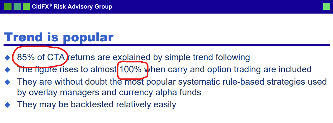 Jessica James was Vice President in CitiFX® Risk Advisory Group Investor Strategy, Citigroup in 2003 (when the remarks were made), and is now the Senior Quantitative Researcher in the Rates Research team at Commerzbank.
4. Rational Expectations
What are Rational Expectations (RE)?
- In modern macroeconomics, the term rational expectations means three things:
- Agents efficiently use all publicly available information (past, present, future).
- Agents understand the structure of the model/economy and base their expectations on this knowledge.
- Therefore, agents can forecast everything with no systematic mistakes.
- The only thing they cannot forecast are the exogenous shocks that hit the economy. These shocks are unpredictable.
- Strong assumptions: the economy’s structure is complex, and nobody truly knows how everything works.
RE are the mathematical expectation of the model
Lots of models in economics take the form: \[y_{t}=x_{t}+\beta \cdot \mathbb{E}_{t} y_{t+1} \tag{4}\]
It says that today’s \(y\) is determined by today’s \(x\) and the expected value of tomorrow’s \(y.\)
What determines this expected value?
Under the RE hypothesis, the agents understand what happens in that process (equation) and formulate expectations in a way that is consistent with it: \[ \mathbb{E}_{t} y_{t+1}=\mathbb{E}_{t} x_{t+1}+\beta \cdot \mathbb{E}_{t} y_{t+2} \tag{5}\]
Eq. (5) is known as the “law of iterated expectations”.
A solution to Rational Expectations
To solve eq. (4), we must iterate forward by inserting eq. (5) into (4). Jump to Appendix B to see how this is done.
At the \(n\)-th iteration, we will get: \[\qquad \qquad \qquad \qquad y_{t}=\sum_{i=0}^{n-1} \beta^{i} \mathbb{E}_{t} x_{t+i} + {\color{blue}\beta^{n} \mathbb{E}_{t} y_{t+n}} \qquad \qquad \qquad \qquad (6)\]
To avoid explosive behavior (secure a stable equilibrium), impose the condition: \[|\beta|<1\]
Which implies that: \[\quad \lim _{n \rightarrow \infty} {\color{blue}\beta^{n} \mathbb{E}_{t} y_{t+n}}=0 \tag{6a}\]
By inserting the result in eq. (6a) into eq. (6), we final get the solution to the stable equilibrium: \[y_{t}=\sum_{i=0}^{n-1} \beta^{i} \mathbb{E}_{t} x_{t+i} \tag{7}\]
But what determines \[\mathbb{E}_{t} x_{t+i}\]
It depends on the nature of the process \(x_t\) itself and how and the type of information we have about \(x_t\)
We discuss this point next.
What determines \(\mathbb{E}_{t} x_{t+i}\)?
- If \(x_t\) is a deterministic process with a steady-sate given by \(\bar{x}\), then: \[\mathbb{E}_{t} x_{t+i}=\bar{x}\]
- If \(x_t\) is a stochastic process, we can compute \(\mathbb{E}_{t} x_{t+i}\) under two different perspectives:
- Unconditional expectations of \(x_t\)
- We only care about the mean of \(x_t\) when formulating expectations
- Conditional expectations of \(x_t\)
- We have specific information about \(x_t\) and we will also use this information
- Unconditional expectations of \(x_t\)
- Next we show how to compute these two expected values.
Unconditional expectations
Suppose that \(x_t\) is given by the following stochastic process:
\[x_{t}=\phi + \rho x_{t-1}+\varepsilon_{t} \ \ , \quad \varepsilon_t \sim \mathcal{N}\left(0, \sigma^2\right) \tag{8}\]The expected-unconditional mean is given by the (deterministic) steady-state value of \(x_t\): \[x_{t}= x_{t-1}= \overline{x}\]
Which leads to: \[\overline{x}=\phi + \rho \overline{x}+0 \Rightarrow \overline{x}=\frac{\phi}{ 1-\rho} \quad , \qquad \rho \neq 1\]
Therefore, the expected (unconditional) value of \(\mathbb{E}_t x_{t+i}\) is given by: \[\mathbb{E}_t x_{t+i}=\overline{x}=\frac{\phi}{ 1-\rho} \tag{9}\]
Conditional expectations
Consider the same stochastic process as in eq. (8):
\[x_{t}=\phi + \rho x_{t-1}+\varepsilon_{t} \ \ , \quad \varepsilon_t \sim \mathcal{N}\left(0, \sigma^2\right) \tag{8'}\]The expected-conditional mean is given by: (for details Jump to Appendix E) \[\mathbb{E}_t x_{t+i}=\sum_{k=0}^{k-1} \phi \rho^k +\rho^i x_t=\frac{\phi}{1-\rho}+\rho^{i} x_t\tag{10}\]
But as \(\bar{x}=\frac{\phi}{1-\rho}\), assuming that \(|\rho|<1\)>, then we can rewrite (10) as: \[\mathbb{E}_t x_{t+i}=\underbrace{\frac{\phi}{1-\rho}}_{\bar{x}}+\underbrace{\rho^i x_t}_{x^\varepsilon}=\bar{x}+ \rho^i x_t^\varepsilon \tag{11}\]
Where \(x^\varepsilon\) is the random component of this process affecting \(x_t\).
Solution: Conditional/Unconditional Expectations
The solution to eq. (7) with unconditional expectations: insert eq. (8) into (7).
The solution to eq. (7) with conditional expectations: insert eq. (11) into (7).
The solution with unconditional expectations is given by: \[y_{t}=\sum_{i=0}^{n-1} \beta^{i} \mathbb{E}_{t} x_{t+i} = \sum_{i=0}^{n-1} \beta^{i}{\overline{x}} =\frac{\overline{x}}{1-\beta}\tag{12}\]
The solution with conditional expectations is given by: \[y_{t}=\sum_{i=0}^{n-1} \beta^{i} \mathbb{E}_{t} x_{t+i} =\sum_{i=0}^{n-1} \beta^i\left[\bar{x}+\rho^i x^\varepsilon_t\right] =\sum_{i=0}^{n-1}\left[\beta^i \bar{x}+\beta^i \rho^i x^\varepsilon_t\right] =\frac{\bar{x}}{1-\beta}+\frac{x^\varepsilon_t}{1-\beta \rho} \tag{13}\]
Empirical Relevance of RE
- In the early 1970s, Robert E. Lucas and Thomas Sargent published a series of papers that created a revolution in macroeconomics.
- They argued that most macroeconomic behavior depends on expectations, and adaptive expectations (AE) was a poor framework.
- The criticisms were already mentioned above:
- AE uses only one type of information (past), which is not rational.
- AE leads to systematic mistakes … which does not make sense.
- They proposed the concept of RE that we have been discussing here.
- How well does such a concept perform when confronted with evidence?
- Let’s see if people, by using all relevant information, make systematic mistakes.
Michigan Survey on Inflation Expectations

The most cited survey in macroeconomics: Michigan Survey
Michigan Survey on Inflation Expectations (cont.)

Most people make systematic mistakes about inflation expectations.
.
MICH performs quite poorly.
Survey of Professional Forecasters (SPF)

The SPF is another major survey on inflation expectations.
.
Data is collected by the Philadelphia Fed.
Survey of Professional Forecasters (cont.)

The SPF produces unbiased expectations, and gives support to RE.
People who use all relevant information do not make systematic mistakes.
4. Summary - Stability Conditions
Predetermined (or backward-looking) variables
A process is called predetermined if its deterministic part depends only upon past observations:
\[x_{t+1}=\phi + \rho x_{t}+\varepsilon_{t+1} \ , \quad \varepsilon \sim i.i.d.(0,\sigma^2)\]Its dynamics will be expressed at the \(n\)-th iteration by: (jump to Appendix C for details) \[\tag{14} x_t={\color{blue}\rho^n x_{t-n}}+\sum_{i=0}^{n-1} \rho^i \phi+\sum_{i=0}^{n-1} \rho^i \varepsilon_{t-i}\]
If \(|\rho|<1 :\) stable solution If \(|\rho|>1 :\) no stable solution If \(|\rho|=1 :\) no solution
Forward-looking variables
A process is called forward-looking if its behavior depends on expected future realizations of its own or of any other variable:
\[y_{t}=x_{t}+\beta \cdot \mathbb{E}_{t} y_{t+1}\]Its dynamics will be expressed at the \(n\)-th iteration by: \[ y_{t}=\sum_{i=0}^{n-1} \beta^{i} \mathbb{E}_{t} x_{t+i} + {\color{blue}\beta^{n} \mathbb{E}_{t} y_{t+n}} \tag{15}\]
If \(|\beta|<1 :\) stable solution
If \(|\beta| >1 :\) no stable solution
If \(|\beta|=1 :\) no solution
Forward-looking variables: a twist
Models with RE are difficult (if not impossible) to solve by pencil and paper.
We have to resort to the computer to “approximate” a solution for us.
We have to write the model with all \(t+1\) variables on the left-hand side of the state-space representation of the system, and those with \(t\) on its right-hand side.
In this case, instead of using the equation: \(y_{t}=x_{t}+\beta \cdot \mathbb{E}_{t} y_{t+1}\)
We should use instead: \[\mathbb{E}_{t} y_{t+n} = - (1/\beta)x_t + (1/\beta)y_t\]
It is easy to see that if \(|\beta|<1\), then \(|1/\beta| >1\): stability condition is the inverse.
Therefore, if the model is written in this way, stability requires \(|1/\beta| >1.\)
5. What is expecting us … ahead
A model with forward & backward-looking behavior
\[\begin{array}{lll} IS: & \hat{y}_{t} =\mathbb{E}_{t} \hat{y}_{t+1}-\frac{1}{\sigma}\left(i_{t}-\mathbb{E}_{t} \pi_{t+1}-r_{t}^{n}\right)+u_t \\ AS: & \pi_{t} =\mu \pi_{t-1}+\kappa \hat{y}_{t}+\beta \mathbb{E}_{t} \pi_{t+1} +s_t \\ MP: & i_{t}=\pi_{t}+r_{t}^{n}+ \phi_{\pi}\left(\pi_{t}-\pi_{t}^{*}\right)+\phi_{y} \hat{y}_{t} \\ \text {Shocks : } & r_{t}^{n} =\rho_r \cdot r_{t-1}^{n}+\varepsilon^r_{t} \ , \quad u_{t} =\rho_u \cdot u_{t-1}+\varepsilon^u_{t} \ , \quad s_{t} =\rho_s \cdot s_{t-1}+\varepsilon^s_{t} \end{array}\] * \(\{i,r_t^n,\hat{y},\pi, u_t, s_t,\varepsilon_t\}\): nominal interest rate, natural real interest rate, output-gap, inflation rate, demand shock, supply shock, and a random disturbance. * \(\{\sigma,\mu, \kappa, \beta,\phi_{\pi},\phi_{y},\pi_{t}^{*},\rho\}\) are parameters * Forward-looking variables: \(\hat{y}_{t}, \pi_{t}\) * Backward-looking variables: \(r_{t}^{n},u_t,s_t\) * Static variables: \(i_t\) * How can we solve this model? Using a computer. Next!
5. Readings
- There is no compulsory reading for this session. We hope that the slides and the notebook will be sufficient to provide a good grasp of the two types of expectations in macroeconomics.
- Many textbooks deal with this subject in a way that is not very useful for our course. They treat this subject in an elementary way or offer a very sophisticated presentation, usually extremely mathematical but short on content.
- There is a textbook that feels quite good for our level: Patrick Minford and David Peel (2019). Advanced Macroeconomics: Primer, Second Edition, Edward Elgar, Cheltenham.
- Chapter 2 deals extensively with AE and RE. However, the former chapter is quite long (40 pages), making it more suitable to be used as complementary material rather than as compulsory reading. But it is by far the best treatment of this subject at this level.
Another excellent treatment of AE and RE can be found in the textbook:
Ben J. Heijdra (2017). Foundations of Modern Macroeconomics. Third Edition, Oxford UP, Oxford.
Chapter 5 deal with this topic at great length (40 pages), but the subject is discussed at a
Appendix A
A step-by-step derivation of equation (2) in the next slide
\[ \begin{aligned} &P_{t}^{e}=\alpha P_{t-1}+(1-\alpha) P_{t-1}^{e}\\ &\downarrow \qquad \qquad \qquad \qquad \quad \ \nwarrow P_{t-1}^{e}=\alpha P_{t-2}+(1-\alpha) P_{t-2}^{e}\\ &P_{t}^{e}=\alpha P_{t-1}+(1-\alpha)\left[\alpha P_{t-2}+(1-\alpha) P_{t-2}^{e}\right]\\ &P_{t}^{e}=\alpha P_{t-1}+\alpha (1-\alpha) P_{t-2}+(1-\alpha)^{2} P_{t-2}^{e}\\ &\downarrow \qquad \qquad \qquad \qquad \qquad \qquad \qquad \qquad\ \ \ \nwarrow P_{t-2}^{e}=\alpha P_{t-3}+(1-\alpha) P_{t-3}^{e}\\ &P_{t}^{e}=\alpha P_{t-1}+ \alpha (1-\alpha) P_{t-2}+(1-\alpha)^{2}\left[\alpha P_{t-3}+(1-\alpha) P_{t-3}^{e}\right]\\ &P_{t}^{e}=\alpha P_{t-1}+ \alpha (1-\alpha) P_{t-2}+\alpha (1-\alpha)^{2} P_{t-3}+(1-\alpha)^{3} P_{t-3}^{e}\\ &P_{t}^{e}=\sum_{i=0}^{3-1} \alpha(1-\alpha)^{i} P_{t-1-i}+{\color{blue}(1-\alpha)^{3} P_{t-3}^{e}}\\ &\text{iterating backward in time up to the $n$-th iteration}\\ &P_{t}^{e}=\sum_{i=0}^{n-1} \alpha(1-\alpha)^{i} P_{t-1-i}+{\color{blue}(1-\alpha)^{n} P_{t-n}^{e}} \end{aligned} \]
Appendix B
A step-by-step derivation of equation (6) in the next slide
\[ \begin{aligned} (iteration \ 1) \qquad \ \ y_t & =\beta \mathbb{E}_t y_{t+1}+x_t \qquad \qquad \qquad \qquad \qquad \qquad \qquad \qquad \quad \ {\color{red}(t\rightarrow t+1)}\\ &\qquad \qquad \nwarrow \mathbb{E}_{t} y_{t+1} = \beta \mathbb{E}_{t} y_{t+2}+\mathbb{E}_{t} x_{t+1} \qquad {\color{red}\text{(Iterated \ expectations)}} \\ (iteration \ 2) \qquad \ \ y_t & =\beta\left(\beta \mathbb{E}_t y_{t+2}+\mathbb{E}_t x_{t+1}\right)+x_t \\ & =\beta^2 \mathbb{E}_t y_{t+2}+\beta \mathbb{E}_t x_{t+1}+x_t \qquad \qquad \qquad \qquad \ \ {\color{red}(t\rightarrow t+1\rightarrow t+2)}\\ &\qquad \qquad \nwarrow \mathbb{E}_{t} y_{t+2} = \beta \mathbb{E}_{t} y_{t+3}+\mathbb{E}_{t} x_{t+2} \qquad {\color{red}\text{(Iterated \ expectations)}}\\ (iteration \ 3) \qquad \ \ y_t & =\beta^2\left(\beta \mathbb{E}_t y_{t+3}+\mathbb{E}_t x_{t+2}\right)+\beta \mathbb{E}_t x_{t+1}+x_t \qquad \\ & =\beta^3 \mathbb{E}_t y_{t+3}+\beta^2 \mathbb{E}_t x_{t+2}+\beta \mathbb{E}_t x_{t+1}+x_t\\ & =\beta^3 \mathbb{E}_t y_{t+3}+\sum_{i=0}^{3-1} \beta^i \mathbb{E}_t x_{t+i} \qquad \qquad \ \ \ \ \ {\color{red}(t\rightarrow t+1\rightarrow t+2 \rightarrow t+3)}\\ (iteration \ n) \qquad \ \ y_t & = \color{blue}{}\beta^n \mathbb{E}_t y_{t+n} \color{black}{}+\sum_{i=0}^{n-1} \beta^i \mathbb{E}_t x_{t+i} \qquad \qquad \ \ \ \ \ {\color{red}(t\rightarrow t+1\rightarrow \ ... \ \rightarrow t+n)} \\ & =\sum_{i=0}^{n-1} \beta^i \mathbb{E}_t x_{t+i} \ \ , \quad \color{blue}{} \text{as} \ \ \beta<|1| \Rightarrow \beta^n \mathbb{E}_t y_{t+n} \rightarrow 0. \qquad \qquad \end{aligned} \]
Appendix C
A step-by-step derivation of equation (14)
\(x_{t}=\phi+\rho x_{t-1}+\varepsilon_{t} \ \ \ \qquad \quad \qquad \qquad \qquad \quad \qquad\) 1st iteration: \(\ t \rightarrow t-1 \qquad \quad\) \(\downarrow \qquad \qquad \quad \nwarrow x_{t-1}=\phi+\rho x_{t-2}+\varepsilon_{t-1} \ \qquad \quad \quad\) Repeated substitution
\(x_t=\phi+\rho\left[\phi+\rho x_{t-2}+\varepsilon_{t-1}\right]+\varepsilon_{t}\ \ \ \qquad \qquad \qquad\) 2nd iteration: \(\ t-1 \rightarrow t-2\)
\(x_t =\phi+\rho \phi+\rho^{2} x_{t-2}+\rho \varepsilon_{t-1}+\varepsilon_{t} \ \ \ \qquad \qquad \qquad\) \(\downarrow \qquad \qquad \qquad \qquad\nwarrow x_{t-2}=\phi+\rho x_{t-3}+\varepsilon_{t-2}\) \(x_{t} =\color{blue}\rho^0 \phi+\rho^{1} \phi+\rho^{2} \phi+\color{black} \rho^{3} x_{t-3}+ \color{red}\rho^{2} \varepsilon_{t-2}+\rho^{1} \varepsilon_{t-1}+\rho^{0} \varepsilon_{t}\color{black}\)
\[x_{t} = \color{blue} \sum_{i=0}^{3-1} \rho^{i} \phi+ \color{black}\rho^{3} x_{t-3}+ \color{red}\sum_{i=0}^{3-1} \rho^{i} \varepsilon_{t-i} \color{black} \qquad \qquad \qquad \qquad \text{$3$rd iteration:} \ t-2 \rightarrow t-3 \quad \] \(\downarrow\) \[x_{t} = \color{blue} \sum_{i=0}^{n-1} \rho^{i} \phi+ \color{black}\rho^{n} x_{t-n}+ \color{red}\sum_{i=0}^{n-1} \rho^{i} \varepsilon_{t-i} \color{black} \qquad \qquad \qquad \qquad \text{$n$th iteration:} \ ... \ {t-n}\qquad\]
Appendix D
A step-by-step derivation of a similar process to that in Appendix B, but now with a constant \({\color{blue} \alpha}\) added to that process:
\[y_{t} = {\color{blue} \alpha} + \beta \mathbb{E}_{t} y_{t+1}+x_{t}\]
See next slide.
\(y_{t} = \alpha+\beta \mathbb{E}_{t} y_{t+1}+x_{t}\) \(\qquad \qquad \qquad \qquad \qquad \qquad \qquad\) 1st iteration: \(\quad t \rightarrow t+1\) \(\downarrow \qquad \qquad \qquad \nwarrow \mathbb{E}_{t} y_{t+1} = \alpha+\beta \mathbb{E}_{t} y_{t+2}+\mathbb{E}_{t} x_{t+1} \ \ \quad \quad \qquad\) Iterated expectations \(y_{t} =\alpha+\beta\left[\alpha+\beta \mathbb{E}_{t} y_{t+2}+\mathbb{E}_{t} x_{t+1}\right]+x_{t} \ \ \ \quad \quad \qquad \quad\) 2nd iteration: \(\ t+1 \rightarrow t+2\) \(y_{t} = \alpha+\beta \alpha+\beta^{2} \mathbb{E}_{t} y_{t+2}+\beta \mathbb{E}_{t} x_{t+1}+x_{t} \ \ \quad \quad \qquad \quad\) \(\downarrow \qquad \qquad \qquad \qquad \quad \nwarrow \mathbb{E}_{t} y_{t+2}=\alpha+\beta \mathbb{E}_{t} y_{t+3}+\mathbb{E}_{t} x_{t+2}\) \(y_{t} = \color{blue}\beta^0 \alpha+\beta^{1} \alpha+\beta^{2} \alpha+ \color{black}\beta^{3} \mathbb{E}_{t} y_{t+3}+ \color{red} \beta^{2} \mathbb{E}_{t} x_{t+2}+\beta^{1} \mathbb{E}_{t} x_{t+1}+\beta^{0} \mathbb{E}_{t} x_{t}\color{black}\) \[y_{t} = \color{blue}\sum_{i=0}^{3-1} \beta^{i} \alpha+ \color{black}\beta^{3} \mathbb{E}_{t} y_{t+3}+ \color{red} \sum_{i=0}^{3-1} \beta^{i} \mathbb{E}_{t} x_{t+i} \color{black} \qquad \qquad \quad \text{3rd iteration:} \ {t+2} \rightarrow {t+3}\] \[y_{t} =\color{blue}\sum_{i=0}^{n-1} \beta^{i} \alpha+ \color{black} \beta^{n} \mathbb{E}_{t} y_{t+n}+ \color{red} \sum_{i=0}^{n-1} \beta^{i} \mathbb{E}_{t} x_{t+i}\color{black} \qquad \qquad \qquad \text{$n$th iteration:} \ ... \rightarrow {t+n}\]
Appendix E
A step-by-step derivation of equation (11)
Apply the expectations operator up to third iteration to:
\(\qquad x_t= \phi+\rho x_{t-1}+\varepsilon_t\)
\(\mathbb{E}_t x_{t+1}=\phi+\rho \mathbb{E}_t x_t+\mathbb{E}_t \varepsilon_{t+1}=\phi+\rho x_t+0=\phi+\rho x_t\)
\(\mathbb{E}_t x_{t+2}=\phi+\rho \mathbb{E}_t x_{t+1}+\mathbb{E}_t \varepsilon_{t+2}=\phi+\rho\left[\phi+\rho x_t\right]+0=\phi+\rho \phi+\rho^2 x_t\)
\(\mathbb{E}_t x_{t+3}=\phi+\rho \mathbb{E}_t x_{t+2}+\mathbb{E}_t \varepsilon_{t+3}=\phi+\rho\left[\phi+\rho \phi+\rho^2 x_t\right] +0 = \underbrace{\phi+\rho \phi+\rho^2 \phi}_{=\sum_{k=0}^{3-1} \phi \rho^k}+ \rho^3x_t\)
Then, generalize to the \(i\)th iteration \[\mathbb{E}_t x_{t+i}=\sum_{k=0}^{k-1} \phi \rho^k +\rho^i x_t=\frac{\phi}{1-\rho}+\rho^{i} x_t\]
Appendix A-2
A step-by-step derivation of equation (2) in the next slide
Let us start: 1st iteration
\(P_{t}^{e}=\alpha P_{t-1}+(1-\alpha) P_{t-1}^{e}\)
Moving 1 period backward
\(P_{t}^{e}=\alpha P_{t-1}+(1-\alpha) P_{t-1}^{e}\)
\(\color{gray} \downarrow \qquad \qquad \qquad \qquad \qquad \ \nwarrow P_{t-1}^{e}=\alpha P_{t-2}+(1-\alpha) P_{t-2}^{e}\)
Let’s get the result in the 2nd iteration
\(P_{t}^{e}=\alpha P_{t-1}+(1-\alpha) P_{t-1}^{e}\)
\(\color{gray} \downarrow \qquad \qquad \qquad \qquad \qquad \ \nwarrow P_{t-1}^{e}=\alpha P_{t-2}+(1-\alpha) P_{t-2}^{e}\)
\(P_{t}^{e}=\alpha P_{t-1}+(1-\alpha)\left[\alpha P_{t-2}+(1-\alpha) P_{t-2}^{e}\right]\)
Simplify the result in the 2nd iteration
\(P_{t}^{e}=\alpha P_{t-1}+(1-\alpha) P_{t-1}^{e}\)
\(\color{gray} \downarrow \qquad \qquad \qquad \qquad \qquad \ \nwarrow P_{t-1}^{e}=\alpha P_{t-2}+(1-\alpha) P_{t-2}^{e}\)
\(P_{t}^{e}=\alpha P_{t-1}+(1-\alpha)\left[\alpha P_{t-2}+(1-\alpha) P_{t-2}^{e}\right]\)
\(P_{t}^{e}=\alpha P_{t-1}+\alpha (1-\alpha) P_{t-2}+(1-\alpha)^{2} P_{t-2}^{e}\)
Moving one more period forward
\(P_{t}^{e}=\alpha P_{t-1}+(1-\alpha) P_{t-1}^{e}\)
\(\color{gray} \downarrow \qquad \qquad \qquad \qquad \qquad \ \nwarrow P_{t-1}^{e}=\alpha P_{t-2}+(1-\alpha) P_{t-2}^{e}\)
\(P_{t}^{e}=\alpha P_{t-1}+(1-\alpha)\left[\alpha P_{t-2}+(1-\alpha) P_{t-2}^{e}\right]\)
\(P_{t}^{e}=\alpha P_{t-1}+\alpha (1-\alpha) P_{t-2}+(1-\alpha)^{2} P_{t-2}^{e}\)
\(\color{gray} \downarrow \qquad \qquad \qquad \qquad \qquad \qquad \qquad \qquad \qquad \nwarrow P_{t-2}^{e}=\alpha P_{t-3}+(1-\alpha) P_{t-3}^{e}\)
Let’s get the result in the 3rd iteration
\(P_{t}^{e}=\alpha P_{t-1}+(1-\alpha) P_{t-1}^{e}\)
\(\color{gray} \downarrow \qquad \qquad \qquad \qquad \qquad \ \nwarrow P_{t-1}^{e}=\alpha P_{t-2}+(1-\alpha) P_{t-2}^{e}\)
\(P_{t}^{e}=\alpha P_{t-1}+(1-\alpha)\left[\alpha P_{t-2}+(1-\alpha) P_{t-2}^{e}\right]\)
\(P_{t}^{e}=\alpha P_{t-1}+\alpha (1-\alpha) P_{t-2}+(1-\alpha)^{2} P_{t-2}^{e}\)
\(\color{gray} \downarrow \qquad \qquad \qquad \qquad \qquad \qquad \qquad \qquad \qquad \nwarrow P_{t-2}^{e}=\alpha P_{t-3}+(1-\alpha) P_{t-3}^{e}\)
\(P_{t}^{e}=\alpha P_{t-1}+ \alpha (1-\alpha) P_{t-2}+(1-\alpha)^{2}\left[\alpha P_{t-3}+(1-\alpha) P_{t-3}^{e}\right]\)
Simplify the result in the 3rd iteration
\(P_{t}^{e}=\alpha P_{t-1}+(1-\alpha) P_{t-1}^{e}\)
\(\color{gray} \downarrow \qquad \qquad \qquad \qquad \qquad \ \nwarrow P_{t-1}^{e}=\alpha P_{t-2}+(1-\alpha) P_{t-2}^{e}\)
\(P_{t}^{e}=\alpha P_{t-1}+(1-\alpha)\left[\alpha P_{t-2}+(1-\alpha) P_{t-2}^{e}\right]\)
\(P_{t}^{e}=\alpha P_{t-1}+\alpha (1-\alpha) P_{t-2}+(1-\alpha)^{2} P_{t-2}^{e}\)
\(\color{gray} \downarrow \qquad \qquad \qquad \qquad \qquad \qquad \qquad \qquad \qquad \nwarrow P_{t-2}^{e}=\alpha P_{t-3}+(1-\alpha) P_{t-3}^{e}\)
\(P_{t}^{e}=\alpha P_{t-1}+ \alpha (1-\alpha) P_{t-2}+(1-\alpha)^{2}\left[\alpha P_{t-3}+(1-\alpha) P_{t-3}^{e}\right]\)
\(P_{t}^{e} = \alpha P_{t-1}+ \alpha (1-\alpha) P_{t-2}+\alpha (1-\alpha)^{2} P_{t-3}+\color{blue}{(1-\alpha)^{3} P_{t-3}^{e}}\)
Use \(\sum\) to further simplify things at the 3rd iteration
\(P_{t}^{e}=\alpha P_{t-1}+(1-\alpha) P_{t-1}^{e}\)
\(\color{gray} \downarrow \qquad \qquad \qquad \qquad \qquad \ \nwarrow P_{t-1}^{e}=\alpha P_{t-2}+(1-\alpha) P_{t-2}^{e}\)
\(P_{t}^{e}=\alpha P_{t-1}+(1-\alpha)\left[\alpha P_{t-2}+(1-\alpha) P_{t-2}^{e}\right]\)
\(P_{t}^{e}=\alpha P_{t-1}+\alpha (1-\alpha) P_{t-2}+(1-\alpha)^{2} P_{t-2}^{e}\)
\(\color{gray} \downarrow \qquad \qquad \qquad \qquad \qquad \qquad \qquad \qquad \qquad \nwarrow P_{t-2}^{e}=\alpha P_{t-3}+(1-\alpha) P_{t-3}^{e}\)
\(P_{t}^{e}=\alpha P_{t-1}+ \alpha (1-\alpha) P_{t-2}+(1-\alpha)^{2}\left[\alpha P_{t-3}+(1-\alpha) P_{t-3}^{e}\right]\)
\(P_{t}^{e} = \alpha P_{t-1}+ \alpha (1-\alpha) P_{t-2}+\alpha (1-\alpha)^{2} P_{t-3}+\color{blue}{(1-\alpha)^{3} P_{t-3}^{e}}\)
\[P_{t}^{e}=\sum_{i=0}^{3-1} \alpha(1-\alpha)^{i} P_{t-1-i}+{\color{blue}(1-\alpha)^{3} P_{t-3}^{e}}\]
Generalize to the \(n\)-th iteration
In the previous slide, we iterated backwards in time 3 times.
The result was: \[P_{t}^{e}=\sum_{i=0}^{3-1} \alpha(1-\alpha)^{i} P_{t-1-i}+{\color{blue}(1-\alpha)^{3} P_{t-3}^{e}}\]
Now, it is easy to see that if we iterate \(n\)-times, instead of 3, we will get:
\[P_{t}^{e}=\sum_{i=0}^{n-1} \alpha(1-\alpha)^{i} P_{t-1-i}+{\color{blue}(1-\alpha)^{n} P_{t-n}^{e}}\]
Appendix B-2
A step-by-step derivation of equation (6) in the next slide
Solution: forward iteration
We will solve the following equation by forward iteration: \[y_{t} = \alpha+\beta \mathbb{E}_{t} y_{t+1}+\theta x_{t}\]
Like this, when \(n \rightarrow \infty\):
\(\underbrace{t \rightarrow (t+1)}_{1\text{st iteration}} \rightarrow\) \(\qquad \qquad \qquad \underbrace{(t+1) \rightarrow (t+2)}_{2\text{nd iteration}} \rightarrow\) \(\qquad \qquad \qquad \qquad \qquad \qquad \qquad \qquad \underbrace{(t+2) \rightarrow (t+3)}_{3\text{rd iteration}} \rightarrow ...\) \(\qquad \qquad \qquad \qquad\qquad \qquad \qquad \qquad \qquad \qquad \qquad \qquad \qquad \underbrace{(t+(n-1)) \rightarrow (t+n)}_{n\text{th iteration}}\)
Let’s start: 1st iteration
\(y_{t} = \alpha+\beta \mathbb{E}_{t} y_{t+1}+\theta x_{t}\) \(\ \qquad \qquad \qquad \qquad \qquad \qquad\) 1st iteration: \(t \rightarrow t+1\)
Going 1 period forward
\(y_{t} = \alpha+\beta \mathbb{E}_{t} y_{t+1}+\theta x_{t}\) \(\ \qquad \qquad \qquad \qquad \qquad \qquad\) 1st iteration: \(\quad t \rightarrow t+1\)
\(\color{gray} \downarrow \qquad \qquad \qquad \nwarrow \mathbb{E}_{t} y_{t+1} = \alpha+\beta \mathbb{E}_{t} y_{t+2}+\theta \mathbb{E}_{t} x_{t+1} \qquad \qquad\) 1 period forward
Get the result in the 2nd iteration
\(y_{t} = \alpha+\beta \mathbb{E}_{t} y_{t+1}+\theta x_{t}\) \(\ \qquad \qquad \qquad \qquad \qquad \qquad\) 1st iteration: \(t \rightarrow t+1\)
\(\color{gray} \downarrow \qquad \qquad \qquad \nwarrow \mathbb{E}_{t} y_{t+1} = \alpha+\beta \mathbb{E}_{t} y_{t+2}+\theta \mathbb{E}_{t} x_{t+1} \qquad \qquad\) 1 period forward
\(y_{t} =\alpha+\beta\left[\alpha+\beta \mathbb{E}_{t} y_{t+2}+\theta \mathbb{E}_{t} x_{t+1}\right]+\theta x_{t}\)
Simplify the result in the 2nd iteration
\(y_{t} = \alpha+\beta \mathbb{E}_{t} y_{t+1}+\theta x_{t}\) \(\ \qquad \qquad \qquad \qquad \qquad \qquad\) 1st iteration: \(t \rightarrow t+1\)
\(\color{gray} \downarrow \qquad \qquad \qquad \nwarrow \mathbb{E}_{t} y_{t+1} = \alpha+\beta \mathbb{E}_{t} y_{t+2}+\theta \mathbb{E}_{t} x_{t+1} \qquad \qquad\) 1 period forward
\(y_{t} =\alpha+\beta\left[\alpha+\beta \mathbb{E}_{t} y_{t+2}+\theta \mathbb{E}_{t} x_{t+1}\right]+\theta x_{t}\)
\(y_{t} = \alpha+\beta \alpha+\beta^{2} \mathbb{E}_{t} y_{t+2}+\beta \theta \mathbb{E}_{t} x_{t+1}+\theta x_{t} \ \ \quad \quad \quad\) 2nd iteration: \(\ t+1 \rightarrow t+2\)
Going 2 periods forward
\(y_{t} = \alpha+\beta \mathbb{E}_{t} y_{t+1}+\theta x_{t}\) \(\ \qquad \qquad \qquad \qquad \qquad \qquad\) 1st iteration: \(t \rightarrow t+1\)
\(\color{gray} \downarrow \qquad \qquad \qquad \nwarrow \mathbb{E}_{t} y_{t+1} = \alpha+\beta \mathbb{E}_{t} y_{t+2}+\theta \mathbb{E}_{t} x_{t+1} \qquad \qquad\) 1 period forward
\(y_{t} =\alpha+\beta\left[\alpha+\beta \mathbb{E}_{t} y_{t+2}+\theta \mathbb{E}_{t} x_{t+1}\right]+\theta x_{t}\)
\(y_{t} = \alpha+\beta \alpha+\beta^{2} \mathbb{E}_{t} y_{t+2}+\beta \theta \mathbb{E}_{t} x_{t+1}+\theta x_{t} \ \ \quad \quad \quad\) 2nd iteration: \(\ t+1 \rightarrow t+2\)
\(\color{gray} \downarrow \qquad \qquad \qquad \qquad \quad \nwarrow \mathbb{E}_{t} y_{t+2}=\alpha+\beta \mathbb{E}_{t} y_{t+3}+\theta \mathbb{E}_{t} x_{t+2} \quad\) 2 periods forward
Get the result in the 3rd iteration
\(y_{t} = \alpha+\beta \mathbb{E}_{t} y_{t+1}+\theta x_{t}\) \(\ \qquad \qquad \qquad \qquad \qquad \qquad\) 1st iteration: \(t \rightarrow t+1\)
\(\color{gray} \downarrow \qquad \qquad \qquad \nwarrow \mathbb{E}_{t} y_{t+1} = \alpha+\beta \mathbb{E}_{t} y_{t+2}+\theta \mathbb{E}_{t} x_{t+1} \qquad \qquad\) 1 period forward
\(y_{t} =\alpha+\beta\left[\alpha+\beta \mathbb{E}_{t} y_{t+2}+\theta \mathbb{E}_{t} x_{t+1}\right]+\theta x_{t}\)
\(y_{t} = \alpha+\beta \alpha+\beta^{2} \mathbb{E}_{t} y_{t+2}+\beta \theta \mathbb{E}_{t} x_{t+1}+\theta x_{t} \ \ \quad \quad \quad\) 2nd iteration: \(\ t+1 \rightarrow t+2\)
\(\color{gray} \downarrow \qquad \qquad \qquad \qquad \quad \nwarrow \mathbb{E}_{t} y_{t+2}=\alpha+\beta \mathbb{E}_{t} y_{t+3}+\theta \mathbb{E}_{t} x_{t+2} \quad\) 2 periods forward
\(y_{t} = \color{blue} \quad \alpha +\beta^{1} \alpha+ \beta^{2} \alpha+ \color{black}\beta^{3} \mathbb{E}_{t} y_{t+3}+ \color{red} \theta \beta^{2} \mathbb{E}_{t} x_{t+2}+ \theta \beta^{1} \mathbb{E}_{t} x_{t+1}+\theta \mathbb{E}_{t} x_{t}\color{black}\)
\(y_{t} = \color{blue}\beta^0 \alpha+\beta^{1} \alpha+ \beta^{2} \alpha+ \color{black}\beta^{3} \mathbb{E}_{t} y_{t+3}+ \color{red} \theta \beta^{2} \mathbb{E}_{t} x_{t+2}+ \theta \beta^{1} \mathbb{E}_{t} x_{t+1}+\theta \beta^{0} \mathbb{E}_{t} x_{t}\color{black}\)
Simplify the result in the 3rd iteration
\(y_{t} = \alpha+\beta \mathbb{E}_{t} y_{t+1}+\theta x_{t}\) \(\ \qquad \qquad \qquad \qquad \qquad \qquad\) 1st iteration: \(t \rightarrow t+1\)
\(\color{gray} \downarrow \qquad \qquad \qquad \nwarrow \mathbb{E}_{t} y_{t+1} = \alpha+\beta \mathbb{E}_{t} y_{t+2}+\theta \mathbb{E}_{t} x_{t+1} \qquad\) Law Iterat. expectations
\(y_{t} =\alpha+\beta\left[\alpha+\beta \mathbb{E}_{t} y_{t+2}+\theta \mathbb{E}_{t} x_{t+1}\right]+\theta x_{t}\)
\(y_{t} = \alpha+\beta \alpha+\beta^{2} \mathbb{E}_{t} y_{t+2}+\beta \theta \mathbb{E}_{t} x_{t+1}+\theta x_{t} \ \ \quad \quad \quad\) 2nd iteration: \(\ t+1 \rightarrow t+2\)
\(\color{gray} \downarrow \qquad \qquad \qquad \qquad \quad \nwarrow \mathbb{E}_{t} y_{t+2}=\alpha+\beta \mathbb{E}_{t} y_{t+3}+\theta \mathbb{E}_{t} x_{t+2} \quad\) 2 periods forward
\(y_{t} = \color{blue} \quad \alpha +\beta^{1} \alpha+ \beta^{2} \alpha+ \color{black}\beta^{3} \mathbb{E}_{t} y_{t+3}+ \color{red} \theta \beta^{2} \mathbb{E}_{t} x_{t+2}+ \theta \beta^{1} \mathbb{E}_{t} x_{t+1}+\theta \mathbb{E}_{t} x_{t}\color{black}\)
\(y_{t} = \color{blue}\beta^0 \alpha+\beta^{1} \alpha+ \beta^{2} \alpha+ \color{black}\beta^{3} \mathbb{E}_{t} y_{t+3}+ \color{red} \theta \beta^{2} \mathbb{E}_{t} x_{t+2}+ \theta \beta^{1} \mathbb{E}_{t} x_{t+1}+\theta \beta^{0} \mathbb{E}_{t} x_{t}\color{black}\)
\[y_{t} = \color{blue}\sum_{i=0}^{3-1} \beta^{i} \alpha+ \color{black}\beta^{3} \mathbb{E}_{t} y_{t+3}+ \color{red} \sum_{i=0}^{3-1} \theta \beta^{i} \mathbb{E}_{t} x_{t+i} \color{black} \qquad \qquad\text{3rd iteration:} \ {t+2} \rightarrow {t+3}\]
Generalize to the \(n\)-th iteration
In the previous slide, we iterated forward 3 times.
The result was: \[y_{t} = \color{blue}\sum_{i=0}^{3-1} \beta^{i} \alpha+ \color{black}\beta^{3} \mathbb{E}_{t} y_{t+3}+ \color{red} \sum_{i=0}^{3-1} \theta \beta^{i} \mathbb{E}_{t} x_{t+i}\]
Now, it is easy to see that if we iterate \(n\)-times forward, instead of 3, we will get:
\[y_{t} =\color{blue}\sum_{i=0}^{n-1} \beta^{i} \alpha+ \color{black} \beta^{n} \mathbb{E}_{t} y_{t+n}+ \color{red} \sum_{i=0}^{n-1} \theta \beta^{i} \mathbb{E}_{t} x_{t+i}\]
Appendix C-2
A step-by-step derivation of equation (14) in the following slides
Solution: backward iteration
We will solve the following equation by backward iteration: \[x_{t}=\phi+\rho x_{t-1}+\varepsilon_{t}\]
Like this, when \(n \rightarrow \infty\): \[\underbrace{t \rightarrow (t-1)}_{1\text{st iteration}} \rightarrow \underbrace{(t-1) \rightarrow (t-2)}_{2\text{nd iteration}} \rightarrow \underbrace{(t-2) \rightarrow (t-3)}_{3\text{rd iteration}} \rightarrow ... \rightarrow\underbrace{(t-(n-1)) \rightarrow (t-n)}_{n\text{th iteration}}\]
The strategy is as follows:
- Iterate up to the 3rd iteration: see a pattern at this iteration
- Then, generalize to the \(n\)th iteration
Let us start: 1st iteration
\(x_{t}=\phi+\rho x_{t-1}+\varepsilon_{t} \qquad \qquad \qquad \qquad \qquad \qquad \qquad\) 1st iteration: \(\ t \rightarrow t-1\)
Going 1 period back in time
\(x_{t}=\phi+\rho x_{t-1}+\varepsilon_{t} \qquad \qquad \qquad \qquad \qquad \qquad \qquad\) 1st iteration: \(\ t \rightarrow t-1\)
\(\color{gray} \downarrow \qquad \qquad \qquad \nwarrow x_{t-1}=\phi+\rho x_{t-2}+\varepsilon_{t-1} \ \ \qquad \quad \qquad\) going back 1 period
Let’s get the result in the 2nd iteration
\(x_{t}=\phi+\rho x_{t-1}+\varepsilon_{t} \qquad \qquad \qquad \qquad \qquad \qquad \qquad\) 1st iteration: \(\ t \rightarrow t-1\)
\(\color{gray} \downarrow \qquad \qquad \qquad \nwarrow x_{t-1}=\phi+\rho x_{t-2}+\varepsilon_{t-1} \ \ \qquad \quad \qquad\) going back 1 period
\(x_{t}=\phi+\rho\left[\phi+\rho x_{t-2}+\varepsilon_{t-1}\right]+\varepsilon_{t}\)
Simplify the result in the 2nd iteration
\(x_{t}=\phi+\rho x_{t-1}+\varepsilon_{t} \qquad \qquad \qquad \qquad \qquad \qquad \qquad\) 1st iteration: \(\ t \rightarrow t-1\)
\(\color{gray} \downarrow \qquad \qquad \qquad \nwarrow x_{t-1}=\phi+\rho x_{t-2}+\varepsilon_{t-1} \ \ \qquad \quad \qquad\) going back 1 period
\(x_{t}=\phi+\rho\left[\phi+\rho x_{t-2}+\varepsilon_{t-1}\right]+\varepsilon_{t}\)
\(x_t=\phi+\rho \phi+\rho^{2} x_{t-2}+\rho \varepsilon_{t-1}+\varepsilon_{t} \ \ \ \qquad \quad \qquad\) 2nd iteration: \(\ t-1 \rightarrow t-2\)
Going 2 periods back in time
\(x_{t}=\phi+\rho x_{t-1}+\varepsilon_{t} \qquad \qquad \qquad \qquad \qquad \qquad \qquad\) 1st iteration: \(\ t \rightarrow t-1\)
\(\color{gray} \downarrow \qquad \qquad \qquad \nwarrow x_{t-1}=\phi+\rho x_{t-2}+\varepsilon_{t-1} \ \ \qquad \quad \qquad\) going back 1 period
\(x_{t}=\phi+\rho\left[\phi+\rho x_{t-2}+\varepsilon_{t-1}\right]+\varepsilon_{t}\)
\(x_t=\phi+\rho \phi+\rho^{2} x_{t-2}+\rho \varepsilon_{t-1}+\varepsilon_{t} \ \ \ \qquad \quad \qquad\) 2nd iteration: \(\ t-1 \rightarrow t-2\)
\(\color{gray} \downarrow \qquad \qquad \qquad \qquad \ \nwarrow x_{t-2}=\phi+\rho x_{t-3}+\varepsilon_{t-2} \ \qquad\) going back 2 periods
Let’s get the result in the 3rd iteration
\(x_{t}=\phi+\rho x_{t-1}+\varepsilon_{t} \qquad \qquad \qquad \qquad \qquad \qquad \qquad\) 1st iteration: \(\ t \rightarrow t-1\)
\(\color{gray} \downarrow \qquad \qquad \qquad \nwarrow x_{t-1}=\phi+\rho x_{t-2}+\varepsilon_{t-1} \ \ \qquad \quad \qquad\) going back 1 period
\(x_{t}=\phi+\rho\left[\phi+\rho x_{t-2}+\varepsilon_{t-1}\right]+\varepsilon_{t}\)
\(x_t=\phi+\rho \phi+\rho^{2} x_{t-2}+\rho \varepsilon_{t-1}+\varepsilon_{t} \ \ \ \qquad \quad \qquad\) 2nd iteration: \(\ t-1 \rightarrow t-2\)
\(\color{gray} \downarrow \qquad \qquad \qquad \qquad \ \nwarrow x_{t-2}=\phi+\rho x_{t-3}+\varepsilon_{t-2} \ \qquad\) going back 2 periods
\(x_{t} = \color{blue} \quad \phi+\rho^{1} \phi+\rho^{2} \phi+\color{black} \rho^{3} x_{t-3}+ \color{red}\rho^{2} \varepsilon_{t-2}+\rho^{1} \varepsilon_{t-1}+ \ \ \varepsilon_{t}\color{black}\) \(x_{t} =\color{blue}\rho^0 \phi+\rho^{1} \phi+\rho^{2} \phi+\color{black} \rho^{3} x_{t-3}+ \color{red}\rho^{2} \varepsilon_{t-2}+\rho^{1} \varepsilon_{t-1}+\rho^{0} \varepsilon_{t}\color{black}\)
Simplify the result in the 3rd iteration
\(x_{t}=\phi+\rho x_{t-1}+\varepsilon_{t} \qquad \qquad \qquad \qquad \qquad \qquad \qquad\) 1st iteration: \(\ t \rightarrow t-1\)
\(\color{gray} \downarrow \qquad \qquad \qquad \nwarrow x_{t-1}=\phi+\rho x_{t-2}+\varepsilon_{t-1} \ \ \qquad \quad \qquad\) going back 1 period
\(x_{t}=\phi+\rho\left[\phi+\rho x_{t-2}+\varepsilon_{t-1}\right]+\varepsilon_{t}\)
\(x_t=\phi+\rho \phi+\rho^{2} x_{t-2}+\rho \varepsilon_{t-1}+\varepsilon_{t} \ \ \ \qquad \quad \qquad\) 2nd iteration: \(\ t-1 \rightarrow t-2\)
\(\color{gray} \downarrow \qquad \qquad \qquad \qquad \ \nwarrow x_{t-2}=\phi+\rho x_{t-3}+\varepsilon_{t-2} \ \qquad\) going back 2 periods
\(x_{t} = \color{blue} \quad \phi+\rho^{1} \phi+\rho^{2} \phi+\color{black} \rho^{3} x_{t-3}+ \color{red}\rho^{2} \varepsilon_{t-2}+\rho^{1} \varepsilon_{t-1}+ \ \ \varepsilon_{t}\color{black}\)
\(x_{t} =\color{blue}\rho^0 \phi+\rho^{1} \phi+\rho^{2} \phi+\color{black} \rho^{3} x_{t-3}+ \color{red}\rho^{2} \varepsilon_{t-2}+\rho^{1} \varepsilon_{t-1}+\rho^{0} \varepsilon_{t}\color{black}\)
\[x_{t} = \color{blue} \sum_{i=0}^{3-1} \rho^{i} \phi+ \color{black}\rho^{3} x_{t-3}+ \color{red}\sum_{i=0}^{3-1} \rho^{i} \varepsilon_{t-i} \color{black} \qquad \qquad \qquad \qquad \text{$3$rd iteration:} \ t-2 \rightarrow t-3\]
Generalize to the \(n\)-th iteration
In the previous slide, we iterated backwards 3 times.
The result was: \[x_{t} = \color{blue} \sum_{i=0}^{3-1} \rho^{i} \phi+ \color{black}\rho^{3} x_{t-3}+ \color{red}\sum_{i=0}^{3-1} \rho^{i} \varepsilon_{t-i}\]
Now, it is easy to see that if we iterate \(n\)-times, instead of 3, we will get:
\[x_{t} = \color{blue} \sum_{i=0}^{n-1} \rho^{i} \phi+ \color{black}\rho^{n} x_{t-n}+ \color{red}\sum_{i=0}^{n-1} \rho^{i} \varepsilon_{t-i}\]