The Hodrick-Prescott Filter
Macroeconomics (M8674)
February 2026
Vivaldo Mendes, ISCTE
vivaldo.mendes@iscte-iul.pt
1. Main goal
Main goal of a filter in macroeconomics
In economics, any filter intends to separate a time-series \(y_t\) into a trend \(\tau_t\) and a cyclical component \(\varphi_t\) such that: \[y_t = \tau_t + \varphi_t \tag{1}\]
- The trend is the long-run component of the time series
- The cyclical component is the short-run component of the time series
Therefore, from (1) we get
\[\varphi_t = y_t - \tau_t \tag{2}\]
- The trick is to minimize eq. (2) subject to some given constraint on \(\varphi_t\)
Types of Filters
- There are various approaches to separate the long-run trend from the short-run cyclical component of a time series \(y(t)\) .
- Linear filter
- Linear filter with breaks
- Nonlinear filters
- Nonlinear filters
- Hodrick-Prescott filter (Hodrick & Prescott, 1997)
- Band Pass filter (Baxter & King, 1999)
- Hamilton filter (James Hamilton, 2017)
- … and some others
Don’t trust the internet or chatbots
- If you do not know what you are doing, you will make stupid mistakes
- The internet is full of wrong (or incomplete) information
- Even very respected sources may mislead you:
- Either you know very well what you are doing, or …
2. The Hodrick-Prescott filter (HP)
The HP filter: some intuition
- We have some data: a time series \(y_t\)
- We want to extract a smooth trend \(\tau_t\) from \(y_t\)
- We want the difference between the two \((\varphi_t)\), to be “acceptable” given what we know about booms and recessions: not too large, not too small
- We introduce a parameter (\(\lambda\)) into a minimization problem to achieve that
- The minimization problem with respect to \(\tau_t\) can be written as:
\[\min _{\tau_{t}} \left\{ {\cal{L(\tau)}} =\sum_{t=1}^{n} \underbrace{\left(y_{t}-\tau_{t}\right)^{2}}_{=\varphi_t^2} +\ {\color{blue}\lambda} \sum_{t=2}^{n-1} \underbrace{\left[\left(\tau_{t+1}-\tau_{t}\right)-\left(\tau_{t}-\tau_{t-1}\right)\right]^{2}}_{\text{constraint}}\right\}\]
The HP filter: Special Cases
The value given to parameter \(\lambda\) is a choice of ours:
\[\min _{\tau_{t}} \left\{ {\cal{L(\tau)}} =\sum_{t=1}^{n} \left(y_{t}-\tau_{t}\right)^{2}+\ {\color{blue}\lambda} \sum_{t=2}^{n-1} \left[\left(\tau_{t+1}-\tau_{t}\right)-\left(\tau_{t}-\tau_{t-1}\right)\right]^{2}\right\}\]
- \(\lambda = 0\) \(\Rightarrow\) trivial solution because there are no cycles : \(y_t= \tau_t, \forall t\)
- \(\lambda \rightarrow \infty \Rightarrow\) linear trend leads to huge cycles between \(y_t\) and \(\tau_t\)
- \(\lambda = 1600\) \(\Rightarrow\) duration/amplitude of cycles acceptable for quarterly data
- \(\lambda = 7\) \(\Rightarrow\) duration/amplitude of cycles acceptable for annual data
- There is no “unquestionable” value for \(\lambda\)
The HP Filter: an Example
- Main objective: obtain cycles as % deviations from the trend
- This has an important implication:
- Time series with a trend: apply logs to the data before extracting the trend and the cycles (
lnGDP,lnCPI) - Time series without a clear trend: do not apply logs to the data (
UR)
- Time series with a trend: apply logs to the data before extracting the trend and the cycles (
- Quarterly data:
US_data.csv - A simple example:
- Real GDP (column
GDP) - Consumer Price Index (column
CPI) - Unemployment Rate (column
UR)
- Real GDP (column

Dealing with rows and columns in a matrix
\(~~~~~~~~~~~~\)
Dealing with rows and columns in a dataframe

To select a column:
- Use its header (
GDPin the example) - It is also possible to use its column number (not shown here)
To select rows:
- Use their numbers (1, 2, 3, …)
- Range of numbers (1:4 in the example)
- No number, just the header: all rows are selected
- Use a condition (e.g.
USdata[USdata.CPI .< 0 , :])
Compute the HP trend and cycles: a single variable
\(~~~~~~\)
Compute the HP trend and cycles: an entire data set
\(~~~~~~\)
Business cycles: Inflation and Unemployment
\(~~~~~~~~~~~~~~~~\)The inflation-gap \(~~~~~~~~~~~~~~~~~~~~~~~~~~~~~~~~~~~~~\)The unemployment-gap


The output-gap: logs vs levels
\(~~~~~~\) Correctly measured: using logs \(~~~~~~~~~~~~~~~~~~~\)Incorrectly measured: using levels


3. Use filters with care
Three Major Issues
- There is no perfect filter … but the HP seems very good.
- Measuring Potential GDP and Natural Unemployment is difficult:
- Potential GDP is usually associated with the HP-trend in GDP … but not exclusively.
- The Natural Rate of Unemployment is largely associated with the HP-trend in unemployment.
- The HP filter can be misused for policy purposes:
- The James Bullard 2012 case in the USA is a well-known example.
- The HP filter is very useful but should be used with care.
Limitations of the HP Filter
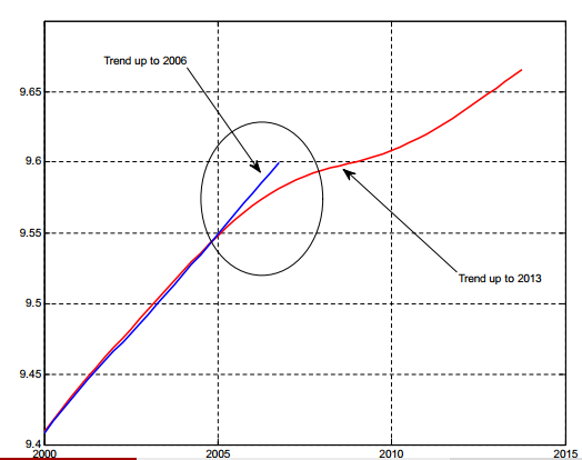
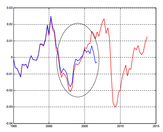
- New data leads to the rewriting of the history of the economy
- The blue lines: data only up to 2008
- The red lines: data up to 2013
| |
|  |
|
Misuses of the HP Filter
- In 2012, the US economy had an unemployment rate close to 8%, one of the highest rates since WWII.
- The Fed Funds Rate was at 0%, to stimulate the economy.
- The inflation rate was much below the target level (2%) at 0.5% and showing signs of going down.
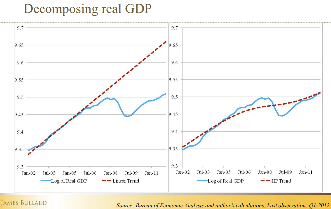
- James Bullard (the President of the Fed of St. Louis), in a famous speech in June 2012 defended that the US economy had gone back to Potential GDP.
- He strongly pushed for a sharp increase in the Fed Funds Rate.
- He used the HP-filter to substantiate his proposal.
The HP filter according to James Bullard
\(~~~~~~~~\)
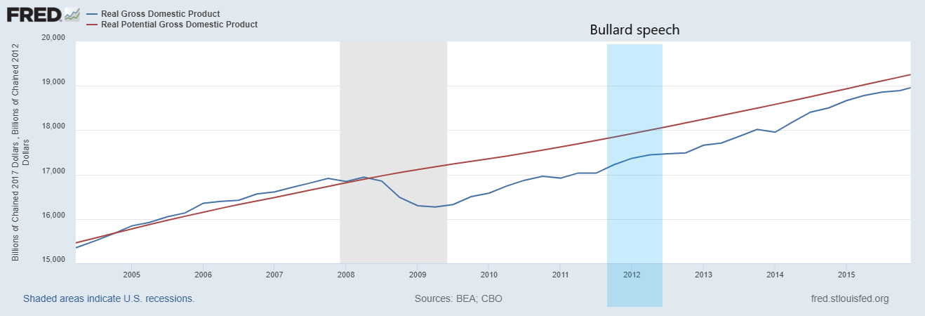
The Output-gap according to the Fed of St. Louis
- The Fed of St. Louis publishes “oficial” US data for Real GDP and Potential GDP.
- Real GDP is the blue line; Potential GDP is the red line.
HP filter & the Natural Unemployment Rate (NUR)
No, Covid-19 did not raise the NUR; no, an increase in NUR did not anticipate Covid-19!

Appendix: HP Filter Derivation
Not compulsory reading
Minimization of the Loss function
The loss function \(\cal{L(\tau)}\) is given by:
\[ \mathcal{L}(\tau)=\sum_{t=1}^n\left(y_t-\tau_t\right)^2+ {\color{blue}\lambda} \sum_{t=2}^{n-1}\left[\left(\tau_{t+1}-\tau_t\right)-\left(\tau_t-\tau_{t-1}\right)\right]^2 \]
To minimize the Loss function with respect to \(\tau_t\):
\[ \min _{\tau_t}\{\mathcal{L}(\tau)\} \]
Take the derivatives with respect to \(\tau_t\) and setting them to zero:
\[ \frac{\partial \mathcal{L}(\tau)}{\partial \tau_t} = 0, \quad \forall t=1, \ldots, n \]
Those derivatives are known as the First Order Conditions (FOCs).
First Order Conditions (FOCs)
- For \(\tau_1:\)
- \({ {\cal{L}}(\tau_1)}=(y_1-\tau_1)^2 +\lambda [\tau_3-2 \tau_2 + \tau_1)]^2\)
- \(\frac{\partial {\cal{L}}(\tau_1)}{\partial \tau_1} = -2\left(y_1-\tau_1\right)+2 \lambda\left(\tau_3-2 \tau_2+\tau_1\right)=0\)
- \((1+\lambda) \tau_1-2 \lambda \tau_2+\lambda \tau_3=y_1 \tag{FOC1}\)
- For \(\tau_2:\)
- \({ {\cal{L}}(\tau_2)}=(y_2-\tau_2)^2 +\lambda [\tau_4- 2 \tau_3 + \tau_2)]^2 + \lambda[(\tau_3-2 \tau_2+\tau_1)]^2\)
- \(\frac{\partial {\cal{L}}(\tau_2)}{\partial \tau_2} = -2\left(y_2-\tau_2\right) + 2 \lambda\left[ \left (\tau_4-2 \tau_3+\tau_2\right) -2\left(\tau_3-2 \tau_2+\tau_1\right)\right]=0\)
- \((1+5 \lambda) \tau_2-2 \lambda \tau_1-4 \lambda \tau_3+\lambda \tau_4=y_2 \tag{FOC2}\)
First Order Conditions (FOCs): continuation
For \(\tau_t\), such that \(t=3, \ldots, n-2\), the FOC is given by:
- \(-2\left(y_t-\tau_t\right)+2 \lambda\left(\tau_{t-2}-4 \tau_{t-1}+6 \tau_t-4 \tau_{t+1}+\tau_{t+2}\right)=0\) or
- \((1+6 \lambda) \tau_t-4 \lambda \tau_{t-1}-4 \lambda \tau_{t+1}+\lambda \tau_{t-2}+\lambda \tau_{t+2}=y_t\)
And for the two right boundary conditions \((n-1, n)\), we have the following FOCs (they are symmetric to those on the left boundary)
- \((1+5 \lambda) \tau_{n-1}-2 \lambda \tau_n-4 \lambda \tau_{n-2}+\lambda \tau_{n-3}=y_{n-1} \tag{FOCn-1}\)
- \((1+\lambda) \tau_n-2 \lambda \tau_{n-1}+\lambda \tau_{n-2}=y_n \tag{FOCn}\)
First Order Conditions (FOCs): Matrix form
The 5 FOCS that represent the optimal conditions on the left boundary, the right boundary, and the interior conditions \((3 \leq t \leq n-2)\) are:
\[
\begin{aligned}
& (1+\lambda) \tau_1-2 \lambda \tau_2+\lambda \tau_3=y_1 \\
& (1+5 \lambda) \tau_2-2 \lambda \tau_1-4 \lambda \tau_3+\lambda \tau_4=y_2 \\
& (1+6 \lambda) \tau_t-4 \lambda\left(\tau_{t-1}+\tau_{t+1}\right)+\lambda\left(\tau_{t-2}+\tau_{t+2}\right)=y_t, \quad 3 \leq t \leq n-2 \\
& (1+5 \lambda) \tau_{n-1}-2 \lambda \tau_n-4 \lambda \tau_{n-2}+\lambda \tau_{n-3}=y_{n-1} \\
& (1+\lambda) \tau_n-2 \lambda \tau_{n-1}+\lambda \tau_{n-2}=y_n
\end{aligned}
\]
So, we can write:
\[ A(\lambda) \tau=y \]
An example with n=6
- \(t=1\)
\(\mathcal{L}(\tau_1)=\left(y_1-\tau_1\right)^2+\lambda\left(\tau_3-2 \tau_2+\tau_1\right)^2\)
\(\frac{\partial \mathcal{L}}{\partial \tau_1}=-2\left(y_1-\tau_1\right)+2 \lambda\left(\tau_3-2 \tau_2+\tau_1\right)=0\)
\((1+\lambda) \tau_1-2 \lambda \tau_2+\lambda \tau_3=y_1\)
- \(t=2\)
\(\mathcal{L}(\tau_2)=\left(y_2-\tau_2\right)^2+\lambda\left(\tau_4-2 \tau_3+\tau_2\right)^2+\lambda\left(\tau_3-2 \tau_2+\tau_1\right)^2\)
\(\frac{\partial \mathcal{L}}{\partial \tau_2}=-2\left(y_2-\tau_2\right) + 2\lambda [\left(\tau_4- 2 \tau_3+\tau_2\right) - 2 \left(\tau_3-2 \tau_2+\tau_1\right)] =0\)
\((1+5 \lambda) \tau_2-2 \lambda \tau_1-4 \lambda \tau_3+\lambda \tau_4=y_2\)
An example with n=6 (cont.)
- \(t=3\)
\(\mathcal{L}(\tau_3)=\left(y_3-\tau_3\right)^2 +\lambda\left(\tau_5-2 \tau_4+\tau_3\right)^2 +\lambda\left(\tau_4-2 \tau_3+\tau_2\right)^2 +\lambda\left(\tau_3-2 \tau_2+\tau_1\right)^2\)
\(\frac{\partial \mathcal{L}}{\partial \tau_3}=-2\left(y_3-\tau_3\right)+2 \lambda\left[\left(\tau_5-2 \tau_4+\tau_3\right) -2\left(\tau_4-2 \tau_3+\tau_2\right)+ \left(\tau_3-2 \tau_2+\tau_1\right)\right]\)
\((1+6 \lambda) \tau_3-4 \lambda \tau_2-4 \lambda \tau_4+\lambda \tau_1+\lambda \tau_5=y_3\)
- \(t=4\)
\(\begin{array}{r}\mathcal{L}\left(\tau_4\right)=\left(y_4-\tau_4\right)^2+\lambda\left(\tau_6-2 \tau_5+\tau_4\right)^2+\lambda\left(\tau_5-2 \tau_4+\tau_3\right)^2+\lambda\left(\tau_4-2 \tau_3+\tau_2\right)^2+ \\ \lambda\left(\tau_3-2 \tau_2+\tau_1\right)^2\end{array}\)
\(\frac{\partial \mathcal{L}}{\partial \tau_4}=-2\left(y_4-\tau_4\right)= 2\lambda [\left(\tau_6-2 \tau_5+\tau_4\right) -2\left(\tau_5-2 \tau_4+\tau_3\right)+ \left(\tau_4-2 \tau_3+\tau_2\right)]=0\)
\((1+6 \lambda) \tau_4-4 \lambda \tau_3-4 \lambda \tau_5+\lambda \tau_2+\lambda \tau_6=y_4\)
An example with n=6 (cont.)
- \(t=5\)
\(\mathcal{L}(\tau_5)=\left(y_5-\tau_5\right)^2 +\lambda\left({\color{blue}\tau_7}-2 \tau_6+\tau_5\right)^2 +\lambda\left(\tau_6-2 \tau_5+\tau_4\right)^2 + ...\)
- This is not a viable way to writing down the Lagrangian function to minimize the problem because \(\tau_7\) is not an interior index, as we have only 6 observations.
- We have to apply the boundary condition that the number of observations end at \(t=6.\)
- Then we will move backward to \(t=5\).
- When we get the results for \(\tau_6\) and \(\tau_5\), the entire solution set is known.
An example with n=6 (cont.)
At the initial boundary we iterate forward, at the end boundary we iterate backwards
- \(t=6\)
\(\mathcal{L}(\tau_6)=\left(y_6-\tau_6\right)^2+\lambda\left(\tau_6-2 \tau_5+\tau_4\right)^2\)
\(\frac{\partial \mathcal{L}}{\partial \tau_6}=-2\left(y_6-\tau_6\right)+2 \lambda\left(\tau_6-2 \tau_5+\tau_4\right)=0\)
\((1+\lambda) \tau_6-2 \lambda \tau_5+\lambda \tau_4=y_6\)
- \(t=5\)
\(\mathcal{L}(\tau_5)=\left(y_5-\tau_5\right)^2+\lambda\left(\tau_5-2 \tau_4+\tau_3\right)^2+\lambda\left(\tau_6-2 \tau_5+\tau_4\right)^2\)
\(\frac{\partial \mathcal{L}}{\partial \tau_5}=-2\left(y_5-\tau_5\right)+2 \lambda\left[\left(\tau_5 - 2 \tau_4+\tau_3\right) - 2\left(\tau_6 -2 \tau_5+\tau_4\right)\right]\)
\((1+5 \lambda) \tau_5-4 \lambda \tau_4-2 \lambda \tau_6+\lambda \tau_3=y_5\)
An example with n=6: all FOCs
\(t=1 \rightarrow (1+\lambda) \tau_1-2 \lambda \tau_2+\lambda \tau_3=y_1\) \(t=2 \rightarrow (1+5 \lambda) \tau_2-2 \lambda \tau_1-4 \lambda \tau_3+\lambda \tau_4=y_2\) \(t=3 \rightarrow (1+6 \lambda) \tau_3-4 \lambda \tau_2-4 \lambda \tau_4+\lambda \tau_1+\lambda \tau_5=y_3\) \(t=4 \rightarrow (1+6 \lambda) \tau_4-4 \lambda \tau_3-4 \lambda \tau_5+\lambda \tau_2+\lambda \tau_6=y_4\) \(t=5 \rightarrow (1+5 \lambda) \tau_5-4 \lambda \tau_4-2 \lambda \tau_6+\lambda \tau_3=y_5\) \(t=6 \rightarrow (1+\lambda) \tau_6-2 \lambda \tau_5+\lambda \tau_4=y_6\)
An example with n=6
If n = 6, the dense form of A is given by: \[ A=\left[\begin{array}{cccccc} 1+\lambda & -2 \lambda & \lambda & 0 & 0 & 0 \\ -2 \lambda & 1+5 \lambda & -4 \lambda & \lambda & 0 & 0 \\ \lambda & -4 \lambda & 1+6 \lambda & -4 \lambda & \lambda & 0 \\ 0 & \lambda & -4 \lambda & 1+6 \lambda & -4 \lambda & \lambda \\ 0 & 0 & \lambda & -4 \lambda & 1+5 \lambda & -2 \lambda \\ 0 & 0 & 0 & \lambda & -2 \lambda & 1+\lambda \end{array}\right] \]
Notice the symmetry of matrix A
- \(diag_2 = [λ, λ, λ, λ]\).
- \(diag_1 = [-2λ, -4λ, -4λ, -4λ, -2λ]\),
- \(diag_0 = [1+λ, 1+5λ, 1+6λ, 1+6λ, 1+5λ, 1+λ]\),
Notebook implementation
- Matrix A non-trivial diagonals:
- \(diag_2 = [λ, λ, λ, λ]\).
- \(diag_1 = [-2λ, -4λ, -4λ, -4λ, -2λ]\),
- \(diag_0 = [1+λ, 1+5λ, 1+6λ, 1+6λ, 1+5λ, 1+λ]\),
- \(diag_{-1} = [-2λ, -4λ, -4λ, -4λ, -2λ]\),
- \(diag_{-2} = [λ, λ, λ, λ]\).
- Check the function
hp_trendin the notebookHP_IRF_2026.jl
4. Readings
Point 2
For this point, there is no compulsory reading.
However, Dirk Krueger (2007). “Quantitative Macroeconomics: An Introduction” (Chapter 2), manuscript, Department of Economics University of Pennsylvania, is well suited for the material covered here.
This text is a small one (12 pages), easy to read, and beneficial for studying the stylized facts of business cycles, mainly to understand how the Hodrick-Prescott filter is calculated. However, notice that, as mentioned, it is not compulsory reading.
Point 3
- No textbook covers the topics/controversies mentioned in this section.
- This coursework intends to provide a framework for a better understanding of these controversies at the end of the course.
- All we have to handle is:
- A little bit of mathematics
- A little bit of computation
- A little bit of macroeconomics