The New Keynesian Model
Macroeconomics (M8674), May 04, 2026
Vivaldo Mendes, ISCTE-IUL
vivaldo.mendes@iscte-iul.pt
1. Introduction
What is the New Keynesian Model (NKM)?
- It’s a DSGEM
- It is a new version of the Old Keynesian model, which was:
- Based on the main ideas of John M. Keynes from the 1930s
- Dominant until the late 1970’s
- Using AE (Adaptive Expectations)
- Based on price and wage rigidities
- The NKM incorporates:
- Adaptive and Rational Expectations
- Allows for price and wage rigidities
- Requires the computer
Is the NKM Relevant today?
” A Google search for the exact phrase “New Keynesian Model” typically yields hundreds of thousands to over a million results, covering academic papers, textbooks, and educational resources … On Google Scholar, the number of results for this specific term exceeds 100,000, confirming its status as a foundational framework in modern macroeconomics.”
From a Google search
“The New Keynesian model arguably remains the dominant framework in the classroom, in academic research, and in policy modeling.”
2. The Structure of the NKM
The IS curve
\[\color{red} \hat{y}_{t}= \mathbb{E}_{t} \hat{y}_{t+1}-\frac{1}{\sigma}\left(i_{t}-\mathbb{E}_{t} \pi_{t+1}-r^{n}\right)+u_t\]
- \(\hat{y}_{t}\) represents the output-gap (% deviations of GDP from Potential GDP).
- \(\mathbb{E}_{t}\) is the conditional expectations operator.
- \(i_t\) is the short term nominal interest rate determined by the central bank.
- \(\mathbb{E}_{t} \pi _{t+1}\) is the level of expected inflation for period \(t+1\).
- \(r^{n}\) is the natural level of the real interest rate (an exogenous variable).
- \(u_t\) is a demand shock.
- \(\sigma\) is a parameter (coefficient of relative risk aversion).
The AS curve
\[\color{red} \pi_{t}=\kappa \cdot \hat{y}_{t} +\beta \cdot \mathbb{E}_{t} \pi_{t+1}+s_t\]
- \(\pi\) is the inflation rate
- \(\hat{y}_{t}\) is the output-gap
- \(s_t\) is a supply shock
- \(\kappa , \beta\) are parameters.
- \(\kappa\) gives the level of price rigidity in the economy:
- \(\kappa \rightarrow \infty\): total flexibility
- \(\kappa \rightarrow 0\): total rigidity
The Monetary Policy Rule
\(~~\) \(~~\) \[\color{red} i_{t}=\pi_{t}+r^{n}+ \phi_{\pi}\left(\pi_{t}-\pi^{_{T}}\right)+\phi_{y} \cdot \hat{y}_{t}+e_t\]
- \(i_t\) is the nominal interest rate determined by the central bank.
- \(\pi_t\) is the inflation rate.
- \(r^{n}\) is the natural level of the real interest rate (exogenous variable)
- \(\pi^{_{T}}\) is the central bank’s target level for the inflation rate (exogenous variable).
- \(e_t\) is a monetary policy shock.
- \(\phi_{\pi}, \phi_y\) are parameters.
- When \(e_t=0\), \(\pi_{t}=\pi^{_{T}}\) and \(\hat{y}_{t}=0\), we have \(i_{t}=\pi_{t}+r^{n}\).
John Taylor (1993). Discretion versus policy rules in practice, Carnegie-Rochester conference series on public policy, 39, 195-214.
Policy Rules and How the Fed Uses Them
- In the website Policy Rules and How Policymakers Use Them, the Fed says they have 5 major rules they use in the decision making process:
- Taylor rule
- Balanced-approach rule
- ELB-adjusted rule
- Inertial rule
- First-difference rule
- The last two perform much better than the others (include a persistence term)
- The Taylor rule is used in this course because it: (i) explains the logic of using rules , and (ii) simplifies the algebra of the NKM
Target Inflation Rate
All central banks in advanced countries have an optimal value for inflation they want to achieve. This is called the inflation target \((\pi^{_{T}})\).
\(~~~~~~~~~~~~~~~~~~~~~~~~~\)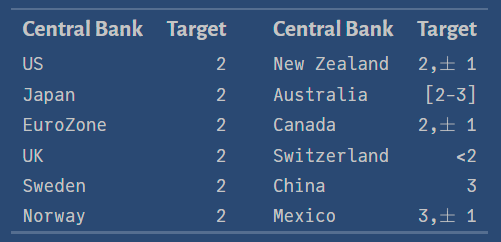
Source: Central Bank News
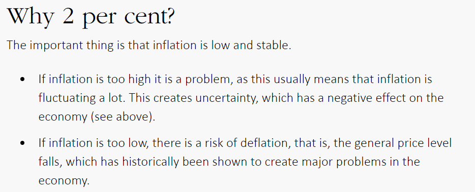
Why 2% Inflation?
According to the Swedish Central Bank (Sveriges Central Bank):
\(~~~~~~~~~\)
The baseline version of the NKM
- The baseline version of the NKM can be simulated with four equations:
\[\begin{array}{lll} IS: & \hat{y}_{t} =\mathbb{E}_{t} \hat{y}_{t+1}-\frac{1}{\sigma}\left(i_{t}-\mathbb{E}_{t} \pi_{t+1}-r^{n}\right)+u_t \\[2pt] AS: & \pi_{t} = \kappa \cdot \hat{y}_{t}+\beta \cdot \mathbb{E}_{t} \pi_{t+1} +s_t \\[2pt] MP: & i_{t}=\pi_{t}+r^{n}+ \phi_{\pi}\left(\pi_{t}-\pi^{_{T}}\right)+\phi_{y} \cdot \hat{y}_{t} + e_t \\[2pt] \text {Shocks : } & u_{t} =\rho_u \cdot u_{t-1}+\varepsilon^u_{t} \ , \quad s_{t} =\rho_s \cdot s_{t-1}+\varepsilon^s_{t} \ , \quad e_{t} =\rho_e \cdot e_{t-1}+\varepsilon^e_{t} \ \\\\ \end{array}\]
- And after this initial simulation, we can simulate the other 3 equations:
\[\begin{array}{lll} \text {Output allocation : } & \hat{y}_{t}= \hat{c}_{t} \\[1pt] \text {Labor supply : } & \hat{\ell}_t=\left(\frac{1-\sigma}{1+\gamma}\right) \hat{y}_t \\[1pt] \text {Technology : } & \hat{a}_t=\left[1-\frac{\alpha(1-\sigma)}{1+\gamma}\right] \hat{y}_t \end{array}\]
An example: the NKM with a demand shock
- The four fundamental equations are:
\[\begin{array}{lllll} \text{Demand shock : } & u_{t+1} =\rho_u u_{t}+\varepsilon_{t+1}^{u} \\[2pt] \text {Taylor rule : } & \ i_{t+1} = \pi_{t+1} + r^n +\phi_{\pi} (\pi_{t+1} - \pi^{_{T}})+\phi_{y} \cdot \hat{y}_{t+1} \\[2pt] \text {AS : } & \pi_{t} =\kappa \cdot \hat{y}_{t}+\beta \cdot \mathbb{E}_{t} \pi_{t+1}\\[2pt] \text {IS : } & \hat{y}_{t}=\mathbb{E}_{t} \hat{y}_{t+1}-\frac{1}{\sigma}\left(i_{t}-\mathbb{E}_{t} \pi_{t+1}-r^{n}\right) + u_t\\[10pt] \end{array}\]
- After solving those four equations, we can also simulate the other three:
\[\begin{array}{lllll} \text {Output allocation : } & \hat{y}_{t}= \hat{c}_{t} \qquad \qquad \qquad \qquad \qquad \qquad \\[2pt] \text {Labor supply : } & \hat{\ell}_t=\left(\frac{1-\sigma}{1+\gamma}\right) \hat{y}_t \\[2pt] \text {Technology : } & \hat{a}_t=\left[1-\frac{\alpha(1-\sigma)}{1+\gamma}\right] \hat{y}_t \\[2pt] \end{array}\]
Matrix representation: the NKM with a demand shock
- The 4 equations can be written as:
\[ \begin{aligned} {\color{blue}1 u_{t+1}+ 0i_{t+1}+ 0 \mathbb{E}_t \pi_{t+1}+0 \mathbb{E}_t \hat{y}_{t+1}} & =\rho_u u_{t}+ 0 i_t + 0 \pi_t+0 \hat{y}_t \ \ \ \ \ \ + {\color{red} 1 \varepsilon_{t+1}^u} \\[3pt] {\color{blue}0 u_{t+1}+ 1i_{t+1}- (1+\phi_\pi) \mathbb{E}_{t} \pi_{t+1}- \phi_y \mathbb{E}_{t}\hat{y}_{t+1}}&=0 u_t + 0 i_t + 0 \pi_t+0 \hat{y}_t \ \ \ \ \ \ \ \ + {\color{red} 0 \varepsilon_{t+1}^i} \ \ + r^n - \phi_\pi \pi^{_T}\\[3pt] {\color{blue}0 u_{t+1}+0 i_{t+1} +\beta \mathbb{E}_t \pi_{t+1}+0 \mathbb{E}_t \hat{y}_{t+1}}&= 0 u_t + 0 i_t +1 \pi_t-\kappa \hat{y}_t \ \ \ \ \ \ \ \ + {\color{red}0 \varepsilon_{t+1}^\pi} \\[3pt] {\color{blue}0 u_{t+1}+0 i_{t+1} +(1/\sigma) \mathbb{E}_t \pi_{t+1}+1 \mathbb{E}_t \hat{y}_{t+1}}&= -1 u_t+ (1/\sigma) i_t + 0 \pi_t+1 \hat{y}_t + {\color{red} 0\varepsilon_{t+1}^y} - (1/\sigma)r^n \\\\ \end{aligned} \]
- Passing the equations into matrices gives:
\[{\color{blue} \underbrace{\left[\begin{array}{cccc} 1 & 0 & 0 & 0 \\ 0 & 1 & -(1+\phi_\pi) & -\phi_y \\ 0 & 0 & \beta & 0 \\ 0 & 0 & \frac{1}{\sigma} & 1 \end{array}\right]}_\mathcal{A}\left[\begin{array}{c}u_{t+1} \\ i_{t+1} \\ \mathbb{E}_t \pi_{t+1} \\ \mathbb{E}_t \hat{y}_{t+1} \end{array}\right]} = \underbrace{\left[\begin{array}{cccc} \rho_s & 0 & 0 & 0 \\ 0 & 0 & 0 & 0 \\ 0 & 0 & 1 & -\kappa \\ -1 & \frac{1}{\sigma} & 0 & 1 \end{array}\right]}_\mathcal{B}\left[\begin{array}{c} u_t \\ i_t \\ \pi_t \\ \hat{y}_t \end{array}\right] + {\color{red} \underbrace{\left[\begin{array}{lll} 1 & 0 & 0 & 0\\ 0 & 0 & 0 & 0\\ 0 & 0 & 0 & 0\\ 0 & 0 & 0 & 0 \end{array}\right]}_{\cal{C}} \left[\begin{array}{c} \varepsilon_{t+1}^{u} \\ \varepsilon_{t+1}^{i} \\ \varepsilon_{t+1}^{\pi} \\ \varepsilon_{t+1}^{y} \end{array}\right]} + \underbrace{\left[\begin{array}{c} \color{teal} 0 \\ \color{teal} r^n - \phi_\pi \pi^{_T} \\ \color{teal} 0 \\ \color{teal} - (1/\sigma) r^n \end{array}\right]}_{\cal{D}}\]
The model is ready for the computer
From the courses’ website, load the Pluto notebook:
- NKM_DemandShock_4x4_NewVersion.jl
Check that the parameters and the matrices are correctly inserted in the notebook
Check the Blanchard-Kahn (BK) conditions
Check the for loops in the notebook
Inspect the IRF of the model and also the impact of the systematic shocks
Check which variables react more to the demand shock.
3. Some (illustrative) results
IRFs from a positive demand shock \((u_1=+1)\)
\(~\)
\(u\): demand shock \(i\): interest rate \(\pi\): inflation rate \(y\): output gap \(\ell\): employment \(a\): technology
IRFs from a negative supply shock \((s_1=+1)\)
\(~\)
\(s\): supply shock \(i\): interest rate \(\pi\): inflation rate \(y\): output gap \(\ell\): employment \(a\): technology
IRFs from the two shocks (demand and supply)
\(~\)
\(u\): demand shock \(s\): supply shock \(i\): interest rate \(\pi\): inflation rate \(y\): output gap \(\ell\): employment \(a\): technology
Time-series from the two shocks
\(~\)
\(u\): demand shock \(s\): supply shock \(i\): interest rate \(\pi\): inflation rate \(y\): output gap \(\ell\): employment \(a\): technology
Heatmap: cross-correlation function (two shocks)
\(~\)
\(u\): demand shock \(s\): supply shock \(i\): interest rate \(\pi\): inflation rate \(y\): output gap \(\ell\): employment \(a\): technology
Standard deviation (two shocks)
\(~~~~~~~~~~~~~~~~~\)
4. Some criticisms of the NKM
Dominant model … but (allegedly) with problems
The first criticism is by the Real Business Cycle people:
- They dislike the rigidity in prices and wages that we find in the NKM
- For them markets are always fully competitive: flexibility in prices and wages.
The second group of criticisms come from inside the NKM literature:
- Counter-intuitive results in the AS curve.
- Counter-intuitive results in the IS curve.
- Lack of persistence
We will discuss this second group of criticisms in the next slides.
Some influential criticisms
The IS and AS curves (allegedly) lead to easily refutable results. See, e.g.:
Ball, L. (1994). “Credible disinflation with staggered price-setting.”American Economic Review, 84(1), 282–289.
Fuhrer, J. and Moore, G. (1995). “Inflation persistence.” Quarterly Journal of Economics, 110(1), 127–159, February.
Fuhrer, J. (1995). The Persistence of Inflation and the Cost of Disinflation, New England Economic Review, January/February 1995, 3-16.
Canzoneri, M. B., Cumby, R. E., and Diba, B. T. (2007). Euler equations and money market interest rates: A challenge for monetary policy models, Journal of Monetary Economics, 54(7), 1863-1881.
Counter-intuitive results in the AS curve
- Consider the AS curve and ignore any shocks \((s_t=0)\):
\(\color{red} \qquad \pi_{t}=\kappa \hat{y}_{t} +\beta \mathbb{E}_{t} \pi_{t+1}+s_t \quad \Rightarrow \quad\pi_{t}- \beta \mathbb{E}_{t} \pi_{t+1}=\kappa \hat{y}_{t} +s_t\)
“If the Federal Reserve engineers a disinflation, it does so by pursuing a contractionary monetary policy that lowers output below potential \((\hat{y}_{t}<0)\). But the flexible inflation model of the equation [above] says that when output falls short of potential, expected inflation in the next period must exceed current inflation. This does not sound like a disinflation”. Fuhrer (1995), page 9
- For simplicity assume \(s_t=0\),\(\ \kappa =1\), \(\beta=1\). A central bank could reduce inflation and produce higher expected inflation at the same time (see next slide for details):
\[ \underbrace{\pi_t-\mathbb{E}_t \pi_{t+1}}_{-2 \%}=\underbrace{\hat{y}_t}_{-2 \%} \]
Furher’s argument in more detail
Suppose the economy is in a stable situation: \(\pi_t = 2\% \ , \ \mathbb{E}_{t} {\pi}_{t+1}=2\% \ , \ \hat{y}_{t}=0\%\) \[\underbrace{\pi_t}_{2\%} - \underbrace{\mathbb{E}_{t} {\pi}_{t+1} }_{2\%} = \underbrace{\hat{y}_{t}}_{0\%} \]
Now, suppose inflation increases to \(3\%\). Normally, higher inflation forces the central bank to increase nominal interest rates, in order to reduce aggregate demand, which in turn will lead to a decrease in inflation and expected inflation.
However, this is not what happens in the AS curve. If inflation goes up to \(3\%\), and the central bank creates a recession of \(\hat{y}_{t}={-1\%}\) , we must get: \[\underbrace{\pi_t}_{3\%} - \underbrace{\mathbb{E}_{t} {\pi}_{t+1} }_{4\%} = \underbrace{\hat{y}_{t}}_{-1\%} \]
It does not make sense: inflation goes up, the central bank creates a recession, and expected inflation goes up. In reality, \(\mathbb{E}_{t} {\pi}_{t+1}\) should go down, not up!
Counter-intuitive results in the IS curve
Consider the IS curve. Put the term \(\mathbb{E}_{t} \hat{y}_{t+1}\) on its left hand side:
\[\color{red} \hat{y}_{t} - \mathbb{E}_{t} \hat{y}_{t+1} = -\frac{1}{\sigma}\left(i_{t}-\mathbb{E}_{t} \pi_{t+1}-r_{t}^{n}\right)+u_t\]
“An awkward implication of [this equation] is that, when the real interest rate rises above its steady-state level, the level of consumption must decrease, but its change must be expected to increase.” Estrella and Furher (2002), page 1021
For simplicity assume \((u_t=0)\) and \(\sigma=1\): The IS seems to give a strange result: \[[(i_{t}-\mathbb{E}_{t} \pi_{t+1}) >r_{t}^{n}] \Rightarrow (\hat{y}_{t} < \mathbb{E}_{t} \hat{y}_{t+1})\]
The central bank may increase \(i_t\) to fight inflation, and the expected output-gap is supposed to increase. Does not make sense (more details in next slide).
Furher&Estrella’s argument in more detail
- Suppose the economy is initially in a stable situation: \(i_t = 3\%, \ , \ \mathbb{E}_{t} {\pi}_{t+1}=2\% \ , r^n_t = 1\% ,\ \hat{y}_{t}=0\%, \mathbb{E}_t \hat{y}_{t+1}=0\%\) \[\underbrace{i_t}_{3\%} - \underbrace{\mathbb{E}_{t} {\pi}_{t+1} }_{2\%} - \underbrace{r^n_t}_{1\%}= -(\underbrace{\hat{y}_{t}}_{0\%} - \underbrace{\mathbb{E}_{t} \hat{y}_{t+1}}_{0\%})\]
- Now, suppose the central bank increases nominal interest rates to \(4\%\). This should lead to the expected output gap to go down, because an increase in \(i_t\) must constrain aggregate demand and economic activity.
- However, that is not what happens in the IS curve:
\[\underbrace{i_t}_{4\%} - \underbrace{\mathbb{E}_{t} {\pi}_{t+1} }_{2\%} - \underbrace{r^n_t}_{1\%}= -(\underbrace{\hat{y}_{t}}_{0\%} - \underbrace{\mathbb{E}_{t} \hat{y}_{t+1}}_{1\%})\]
- An increase in \(i_t\) leads to an increase in the expected output gap: it doses not make sense.
The shapes of the IRFs are wrong in the NKM
- In macroeconomics, most variables respond to a shock gradually.
\(~\)
Their IRFs are hump-shaped, like the one on the left, very different from the NKM ones.
5. Evaluating the Criticisms
Does disinflation lead to higher inflation and output?
- The two arguments by Estrella and Fuhrer can be summarized as follows. Disinflationary measures should lead to:
- higher inflation expectations (AS curve)
- an increase in the expected output gap (IS curve)
- Their arguments are incorrect because they isolate their analysis to equation-by-equation, instead of considering the entire model.
- Suppose there is a positive demand shock that leads to higher inflation and output.
- Then, the central bank raises nominal interest rates to fight inflation.
- The IFRs can be found in the slide below. Anything wrong with them?
- No! In fact in period 2, we have: \({\ \color{red}{\uparrow i_t \ \Rightarrow \ \downarrow \pi, \downarrow \hat{y}}, \ \downarrow \hat{\ell}, \ \downarrow \hat{a}}\)
In period 1, a positive demand shock \((u_{t+1}=1)\) leads to higher inflation; in period 2, the central bank, to fight inflation, sharply raises the nominal interest rate \((e_{t+2}=1)\)
\(~\)
The NKM with inflation and output persistence
- To overcome the problem of hump-shaped IRFs we need to introduce:
- lagged inflation in the AS curve
- lagged output in the IS curve
- lagged interest rates in the MP rule (inertia) as the Fed does
- So the problem is not the model, but omitting fundamental parts of reality.
\[\begin{array}{lll} IS: & \hat{y}_{t} = {\color{red}{\xi \cdot \hat{y}_{t-1}}} + {\color{red}{(1-\xi)}}\mathbb{E}_{t} \hat{y}_{t+1}-\frac{1}{\sigma}\left(i_{t}-\mathbb{E}_{t} \pi_{t+1}-r_{t}^{n}\right)+u_t \\[3pt] AS: & \pi_{t} ={\color{red}{\omega \cdot \pi_{t-1}}}+\kappa \hat{y}_{t}+\beta \mathbb{E}_{t}\pi_{t+1} +s_t \ , \qquad \ {\color{red}{\beta =1-\omega}}\\[3pt] MP: & i_{t}= {\color{red}{\eta \cdot i_{t-1}}}+ \phi_{\pi}\left(\pi_{t}-\pi_{t}^{*}\right)+\phi_{y} \hat{y}_{t} + e_t \\[3pt] \text {Shocks : } & u_{t} =\rho_u u_{t-1}+\varepsilon^u_{t} \ , \quad s_{t} =\rho_s s_{t-1}+\varepsilon^s_{t} \ , \ \ e_{t} =\rho_e e_{t-1}+\varepsilon^e_{t}\\ \end{array}\]
Hump-shaped IRFs in the NKM
\(~\)
- A positive demand shock of \(+1\)
- No more shocks
- \(\omega = 0.9\)
- \(\xi = 0.6\)
- \(\eta=0.25\)
Appendix A
Derivation of the IS Curve (not required in the evaluation process)
Household Utility
Utility of the representative household follows the same beahvior as in the Real Business Cycle model
- It depends positively on real consumption \((c)\) and negatively on hours worked \((\ell)\)
\[u\left(c_t, \ell_t\right)=\frac{c_t^{1-\sigma}}{1-\sigma}-\theta \frac{\ell_t^{1+\gamma}}{1+\gamma} \quad, \quad\{\sigma, \gamma, \theta\} \geq 0 \tag{1}\]
- \(\sigma,\gamma.\theta\) are parameters
- The marginal utility of consumption is given by: \[ u'\left(c_{t}\right)=c_{t}^{-\sigma} \tag{2} \]
- The marginal utility of labor is given by: \[ u^{\prime}\left(\ell_{t}\right)=-\theta \ell_{t}^{\gamma} \tag{3} \]
Firm’s Production Function
- In the baseline version of the NKM, there are no investment expenditures, which means that the capital stock has to be treated as exogenous (or fixed).
- We assume a traditional production function with constant returns to scale, where \(k\) is normalized to 1:
\[y_t = a_t k_t^{(1-\alpha)} \ell_t^\alpha=a_t \ell_t^\alpha\]
- \(y_t\) is output, \(a_t\) is technology, and \(\ell_t\) is hours worked.
- Factor markets are competitive: so the real wage must be equal to the marginal product of labor: \[w_t=\frac{\partial {y}_t}{\partial \ell_t} \Rightarrow w_t=\alpha a_t \ell_t^{\alpha-1}= \alpha \left(\frac{y_t}{\ell_t}\right) \tag{4}\]
Maximization of Utility
- Households maximize utility \((u)\) which depends on consumption \((c)\) and hours worked \((\ell)\) over time
\[\beta^t \cdot u(c_t)+ \beta^{t+1} \cdot\mathbb{E}_{t}u(c_{t+1},\ell_{t+1})+...\]
Subject to a constraint in every period
\[t: \quad \quad \quad \cal{B}_{t} + \cal{P}_{t} c_t = \cal{P}_{t} (\ell_t \cdot w_t) \quad \quad \quad \quad \quad \quad \quad \quad \quad \tag{5}\] \[t+1: \quad \quad \quad \underbrace{{\cal{B}}_{t+1}}_{=0} + {\cal{P}}_{t+1} c_{t+1} = {\cal{P}}_{t+1} (\ell_{t+1} \cdot w_{t+1}) + {\cal{B}}_{t}(1+i_t) \tag{6}\]\(c\) is real consumption, \(\cal{P}\) is the price level, \(w\) is the real wage, \(i\) is the nominal interest rate, and \(\cal{B}\) is the level of nominal bonds
\({\cal{B}}_{t+1}=0\): it does not make sense to have positive savings in some last period
The Lagrangian Function and FOCs
The maximization of utility is given by the Lagrangian function \((\cal{L})\):
\[\max_{c_{t}, \ell_{t}, {\cal{B}}_{t}} {\cal{L}}=\beta^{t}\left[u\left(c_{t}\right)+\lambda_{t}\left(\cal{P}_{t} \ell_t w_t -\cal{P}_{t} c_{t}-{\cal{B}}_{t}\right)\right] + \qquad \qquad \qquad \qquad \]
\[\qquad \quad \quad \beta^{t+1}\left[u\left(c_{t+1}\right)+\lambda_{t+1}\left( {\cal{P}}_{t+1} \ell_{t+1} w_{t+1}- {\cal{P}}_{t+1} c_{t+1}+ (1+i_t) \cal{B}_{t}\right)\right]\]
and the First Order Conditions (FOCs) are: \[ \begin{aligned} \qquad \quad \quad \quad \quad &\frac{\partial \cal{L}}{\partial c_{t}}=0 \Rightarrow \beta^{t}\left [u^{\prime}\left(c_{t}\right)-\lambda_{t} \cal{P}_{t}\right]=0 \Rightarrow {\color{red} u^{\prime}\left(c_{t}\right)/\cal{P}_{t}=\lambda_{t}} \qquad \qquad \qquad \qquad \ \text{(FOC1)}\\ \qquad \quad \quad \quad \quad &\frac{\partial \cal{L}}{\partial \ell_t}=0 \Rightarrow \beta^t\left[u^{\prime}\left(\ell_t\right)-\lambda_t \cal{P}_t w_t\right]=0 \Rightarrow {\color{red} u^{\prime}\left(\ell_t\right)= - \lambda_t \cal{P}_t w_t} \qquad \qquad \qquad \text{(FOC2)}\\ \qquad \quad \quad \quad \quad &\frac{\partial \cal{L}}{\partial \cal{B}_{t}}=0 \Rightarrow-\beta^{t} \lambda_{t}+\beta^{t+1} \lambda_{t+1}\left(1+i_{t}\right)=0 \Rightarrow {\color{red} \lambda_{t}=\beta \lambda_{t+1}\left(1+i_{t}\right)} \quad \quad \quad \ \text{(FOC3)} \end{aligned} \]
The Euler equation and optimal consumption
From FOC1 and FOC3, we have: \[{\color{red} u^{\prime}\left(c_{t}\right)/\cal{P}_{t}=\lambda_{t}} \quad , \quad {\color{red} u^{\prime}\left(c_{t+1}\right)/ {\cal{P}}_{t+1}=\lambda_{t+1}} \quad , \quad {\color{red} \lambda_{t}=\beta \lambda_{t+1}\left(1+i_{t}\right)} \]
From these, we can obtain:
\[\frac{u^{\prime}\left(c_{t}\right)}{\cal{P}_{t}}=\beta \frac{u^{\prime}\left(c_{t+1}\right)}{{\cal{P}}_{t+1}}(1+i_t)\]
simplifying
\[ u^{\prime}\left(c_{t}\right)=\beta \cdot u^{\prime}\left(c_{t+1}\right)(1+i_t)\frac{\cal{P}_{t}}{{\cal{P}}_{t+1}}\]
Now, \(\frac{\cal{P}_{t}}{{\cal{P}}_{t+1}} = \frac{1}{1+\pi_{t+1}}\), where \(\pi_{t+1}\) is the inflation rate at \(t+1\), so:
\[ u^{\prime}\left(c_{t}\right)=\beta \cdot u^{\prime}\left(c_{t+1}\right)\frac{1+i_t}{1+\pi_{t+1}} \tag{7}\]
The optimal labor supply
From FOC2, we have:
\[u^{\prime}\left(\ell_t\right)=-\lambda_t \mathcal{P}_t w_t\]And from FOC1, we got: \(\lambda_t = u'(c_t)/\mathcal{P}_t\)
We know that the marginal utility of consumption is given by eq. (2): \(u'(c_t) = c_t^{-\sigma}\)
We know also that the marginal utility of labor is given by eq. (3): \(u'(\ell_t) = -\theta \ell_t^{\gamma}\)
On the other hand, we know that the real wage is given by the marginal product of labor (see eq. (4)): \(w_t = \alpha \left(\frac{y_t}{\ell_t}\right)\)
Inserting all these results into FOC2, leads to:
\[-\theta \ell_t^{\gamma}= -\left( \frac{u'(c_t)}{\mathcal{P}_t} \right) \mathcal{P}_t \alpha \left(\frac{y_t}{\ell_t}\right) \quad \Rightarrow \quad \theta \ell_t^{\gamma} = c_t^{-\sigma} \alpha \frac{y_t}{\ell_t} \tag{8}\]
Uncertainty and the Euler Equation
The Euler equation, see equation (7) gives the optimal trade-off between consumption today versus consumption in the future:
But the future is not known with certainty, so the variables expressed with \(t+1\) will have to be taken under the expectations operator
\[ u^{\prime}\left(c_{t}\right)=\beta \cdot \mathbb{E}_{t} \left\{ u^{\prime}\left(c_{t+1}\right) \frac{1+i_{t}}{1+\pi_{t+1}} \right\}\]
- But from eq. (2), we know that \(u'(c_t) = c_t^{-\sigma}\). For \(t+1\), we must have that \(u'(c_{t+1}) = c_{t+1}^{-\sigma}\). So, the Euler equation can be written as:
\[ c_{t}^{-\sigma}=\beta \cdot \mathbb{E}_{t}\left\{c_{t+1}^{-\sigma} \left[ \frac{1+i_{t}}{1+\pi_{t+1}} \right] \right\} \tag{9}\]
Applying logs to the Euler equation
- Applying logs to the Euler equation
\[-\sigma \ln c_{t}= \ln \beta + \mathbb{E}_{t}\left\{ -\sigma \ln c_{t+1} + {\color{red} \ln\left[ \frac{1+i_{t}}{1+\pi_{t+1}} \right] } \right\}\]
- If \((i,\pi)\) are small values, then
\[\ln(1+i)\approx i \quad , \quad \ln(1+\pi)\approx \pi\]
- So, the log version of the Euler equation will look like:
\[ -\sigma \ln c_{t}= \ln \beta + \mathbb{E}_{t} (-\sigma \ln c_{t+1} + \underbrace{i_t - \pi_{t+1}}_{r_{t}}) \tag{10}\]
- The Euler eq. in the steady-state (notice that \(r^n_t\) is the natural real interest rate):
\[ -\sigma \ln \overline{c}_{t}= \ln \beta + \mathbb{E}_{t} (-\sigma \ln \overline{c}_{t+1} + r^n_t) \tag{11} \]
Percentage Deviations from the Steady-state
Subtract eq. (11) from (10), and get consumption as a % deviation from steady-state: \[\hat{c}_t = \ln c_t - \ln \overline{c}_{t}\]
Therefore:
\[-\sigma \ln c_{t}-\sigma \ln \overline{c}_{t}= \cancel{\ln \beta} + \mathbb{E}_{t} (-\sigma \ln c_{t+1} + i_t - \pi_{t+1}) - \cancel{\ln \beta} + \mathbb{E}_{t} (-\sigma \ln \overline{c}_{t+1} + r^n_t) \]
\[-\sigma \hat{c}_{t} = \mathbb{E}_{t} (-\sigma \hat{c}_{t+1} + i_{t} - \pi_{t+1} -r^n_t)\]
- That is:
\[ \hat{c}_{t} = \mathbb{E}_{t} \hat{c}_{t+1} - \frac{1}{\sigma} \left( i_{t} - \mathbb{E}_{t} \pi_{t+1} -r^n_t \right) \tag{12}\]
Output allocation
- To make things as easy as possible, consider an economy where output is allocated to consumption and government consumption:
\[ y_t = c_t + g_t \tag{13}\]
\(y_t\) is real GDP, \(c_t\) is real consumption, \(g_t\) stands for real government spending on goods&services.
This means that there are no Investment expenditures, nor Exports or Imports.
Linearizing eq. (13) near the steady-state , we get:
\[{\color{red} \hat {y}_t = \tau \hat {c}_t + (1-\tau)\hat {g}_t} \tag{14}\]
- where \(\tau = \overline{c}/ \overline{y}\) and \((1-\tau) = \overline{g}/\overline{y}\), and \(\overline {c}, \overline {y}, \overline {g}\) are the steady-state values.
The IS function (I)
- The simplest economy of all is one where GDP \((y_t)\) is equal to consumption.
- This is the case when \(\tau=1\) in eq. (14):
\[y_t = c_t \quad \Rightarrow \quad \hat {y}_t = \hat{c}_t \tag{15}\]
- Therefore, by inserting eq. (15) into eq. (12) we obtain the IS function:
\[{\color{red} \hat{y}_{t} = \mathbb{E}_{t} \hat{y}_{t+1} - \frac{1}{\sigma}( i_{t} - \mathbb{E}_{t} \pi_{t+1} -r^n_t)} \tag{16}\]
- The output-gap \((\hat {y}_t)\) depends upon the expected output gap \((\mathbb{E}_{t} \hat{y}_{t+1})\), and the difference between the expected real interest rate \((i_{t} - \mathbb{E}_{t} \pi_{t+1})\) and the natural real interest rate \((r^n_t)\).
The IS function with Government Spending (I)
- Now, consider that \(\tau<1\), implying the existence of public spending.
- To derivate the IS function, insert eq. (12) into (14) which leads to:
\[ \hat{y}_{t}=\tau\left[\mathbb{E}_{t} \hat{c}_{t+1}-\frac{1}{\sigma}\left(i_{t}- \mathbb{E}_{t} \pi_{t+1}-r_{t}^{n}\right)\right]+(1-\tau) \hat{g}_{t} \tag{15} \]
- Then, from eq. (14) we can obtain for period \(t+1\)
\[ \tau \mathbb{E}_{t} \hat{c}_{t+1}=\mathbb{E}_{t} \hat{y}_{t+1}-(1-\tau) \mathbb{E}_{t} \hat{g}_{t+1} \tag{16} \]
- Now, insert eq. (16) into (15), and simplify to obtain the IS function:
\[ {\color{red} \hat{y}_{t}=\mathbb{E}_{t} \hat{y}_{t+1}-\frac{\tau}{\sigma}\left(i_{t}- \mathbb{E}_{t} \pi_{t+1}-r_{t}^{n}\right)+ (1-\tau)\left(\hat{g}_{t}- \mathbb{E}_{t} \hat{g}_{t+1}\right)} \tag{17} \]
The IS function with Government Spending (II)
- Another way of expressing the demand side of the economy is to have two equations (instead of just one, as in eq. 17). These two are:
- The linearized Euler equation:
\[{\color{red} \hat{c}_{t} = \mathbb{E}_{t} \hat{c}_{t+1} - \frac{1}{\sigma} \left( i_{t} - \mathbb{E}_{t} \pi_{t+1} -r^n_t \right)} \tag{12'}\]
- The linearized aggregate demand equation
\[{\color{red} \hat {y}_t = \tau \hat {c}_t + (1-\tau)\hat {g}_t} \tag{14'} \]
- These two equations display the inter-relationships between consumption, output, and government spending, the expected real interest rate, and the natural real interest rate.
The optimal consumption pattern: graphical analysis
\(~~~~~~~~~~~~~~~~\)
Appendix B
Derivation of the AS Curve (not required in the evaluation process)
Price Rigidity: three different ways … similar results
John M. Roberts (1995). “New Keynesian economics and the Phillips curve,” Journal of Money, Credit, and Banking, 27(4), 975–984.
Shows that the 3 papers below lead to similar results:
- John Taylor (1979). “Staggered Wage Setting in a Macro Model,” American Economic Review, P&P, Vol. 69, 108-113.
- Julio Rotemberg (1982), “Monopolistic price adjustment and aggregate output,” Review of Economic Studies, 49(4), 517–531.
- Guillermo Calvo (1983). “Staggered prices in a utility-maximizing framework”, Journal of Monetary Economics, 12(3), 383-398.
We will follow Calvo’s pricing.
Main assumptions: Calvo Pricing
- A1. In each period, a proportion of firms \((\mu)\) do not reset their prices.
- A2. There is monopolistic competition in the goods market: firms set prices (the optimal price, \(p^*_t)\) with a markup \((m_t)\) over marginal costs \((x_t)\). In logs:
\[ p_{t}^{*}=m_{t}+x_{t} \tag{18}\]
- A3. Firms know that the price they set today \((z_t)\) remains constant during some time. So \(z_t\) is set to minimize the profit loss for not resetting prices.
- A4. Real marginal cost in logs \((x_{t}-p_{t})\) depends on the output gap \((\hat{y}_t)\)
\[x_{t}-p_{t}=\psi \hat{y}_t \quad , \quad \psi>0 \tag{19}\]
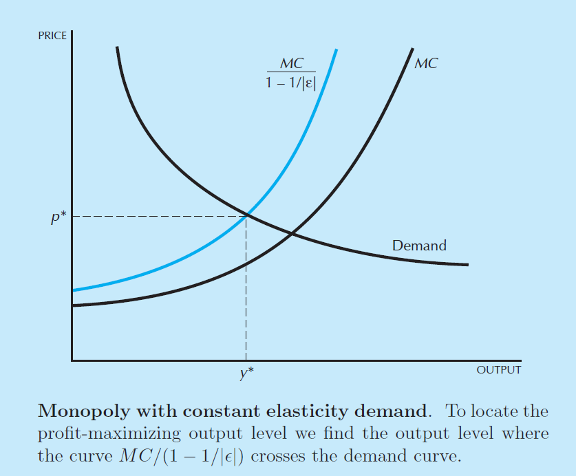
Monopolistic competition pricing
From: Hal Varian (2010). Intermediate Microeconomics: A Modern Approach, 8th Ed.
\(~~~~~~~~~~~~~~~~\)
Minimizing the Loss function
- Given assumptions A1 and A3, the Loss function \(L(z_t)\) is given by
\[ L\left(z_{t}\right)=\sum_{n=0}^{\infty}(\mu \beta)^{n} \cdot \underbrace{\mathbb{E}_{t}\left(z_{t}-p_{t+n}^{*}\right)^{2}}_{\text {expected profit loss}} \tag{20}\]
- \(z_t\) is the (log) price level that minimizes the losses until \(t+n\)
- \(\beta\) is a time discount factor
- \(\mu^n\) is the probability of having the price constant until \(t + n\)
- To minimize \(L(z_t)\)
\[\frac{\partial L}{\partial z_{t}}=0 \Rightarrow 2 \sum_{n=0}^{\infty}(\mu \beta)^{n} \cdot \mathbb{E}_{t}\left(z_{t}-p_{t+n}^{*}\right)=0\]
Minimizing the Loss function (cont.)
\[2 \sum_{n=0}^{\infty}(\mu \beta)^{n} \cdot \mathbb{E}_{t}\left(z_{t}-p_{t+n}^{*}\right)=0\]
\[\underbrace{\sum_{n=0}^{\infty}(\mu \beta)^{n} \cdot z_{t}}_{=\frac{1}{1-\mu \beta} \cdot z_{t}}=\sum_{n=0}^{\infty}(\mu \beta)^{n} \cdot \mathbb{E} p_{t+n}^{*}\]
\[ z_{t}=(1-\mu \beta) \sum_{n=0}^{\infty}(\mu \beta)^{n} \cdot \mathbb{E}_{t} p_{t+n}^{*} \tag{21}\]
The price set by firms \((z_t)\) is an exponential smoothing process of the prices set in the future if there were no price rigidities.
Markup and Marginal Costs
- In eq. (21), \(z_t\) depends on the optimal price level \((p_{t+n}^{*})\).
- But according to A2, the latter depends on the markup \((m)\) and on the marginal cost \((x_t)\)
\[ p_{t}^{*}=m_{t}+x_{t}\]
- Inserting this equation into eq. (21), leads to:
\[ z_{t}=(1-\mu \beta) \sum_{n=0}^{\infty}(\mu \beta)^{n} \cdot \mathbb{E}_{t}\left(m_{t+n}+x_{t+n}\right) \tag{22}\]
- Firms set prices today depending on the expected levels of markups they are able to impose and on the expected levels of marginal costs.
The Aggregate Price level
- In the entire economy, the aggregate price level \((p_t)\) is easy to obtain following assumptions A1 and A3.
- \(\mu\) is the proportion of firms that keep prices unchanged.
- \(1-\mu\) is the proportion of firms that reset current prices.
- Therefore, the aggregate price level in logs \((p_t)\) has to be given by:
\[p_{t}=\mu \cdot p_{t-1}+(1-\mu) \cdot z_{t}\]
- Solving for \(z_t\), leads to:
\[\qquad \qquad \qquad \qquad \qquad z_{t}=\frac{1}{1-\mu}\left(p_{t}-\mu p_{t-1}\right) \tag{23}\]
- \(p_{t-1}\) is the last period’s aggregate price level, \(z_t\) is the new reset price.
A crucial trick
- To write eq. (22) in a more useful manner, we have to apply a trick.
- From the solution to RE models, one may recall that, if we have an equation:
\[y_{t}=a \cdot x_{t}+b \cdot\mathbb{E}_{t} y_{t+1}\]
- … we will get the following solution at the \(n\)-th iteration (provided that \(|b|<1\)):
\[y_{t}=a \sum_{i=0}^{n-1} b^{i} \cdot \mathbb{E}_{t} x_{t+i}\]
- Therefore, as \((|\mu \beta|<1)\), eq. (22) has to be the solution to the equation:
\[ z_{t}=\mu \beta \cdot \mathbb{E}_{t} z_{t+1}+(1-\mu \beta)\left(m_{t}+x_{t}\right) \tag{24}\]
- Now, we can solve our problem, using equations (23) and (24).
Solving the model
- From eq. (23) we get:
\[z_{t}=\frac{1}{1-\mu}\left(p_{t}-\mu p_{t-1}\right)\]
- And from eq. (24) we have:
\[z_{t}=\mu \beta \cdot \mathbb{E}_{t} z_{t+1}+(1-\mu \beta)\left(m_{t}+x_{t}\right)\]
- Equalizing both equations leads to
\[\frac{1}{1-\mu}\left(p_{t}-\mu p_{t-1}\right)=\mu \beta \cdot \frac{1}{1-\mu}\left(\mathbb{E}_{t} p_{t+1}-\mu p_{t}\right)+(1-\mu \beta)\left(m_{t}+x_{t}\right)\]
- Now, we have to simplify this equality:
- Multiply both sides by \(1-\mu\) and subtract \(p_t\) from both sides.
Simplifying
- After multiplying both sides by \(1-\mu\), we will get
\[p_{t}\left(1+\mu^{2} \beta\right)-\mu p_{t-1}=\mu \beta \mathbb{E}_{t} p_{t+1}+(1-\mu)(1-\mu \beta) (m_{t} + x_{t})\]
- After subtracting \(p_t\) from both sides, and defining \(\mathbb{E}_{t} \pi_{t+1} = \mathbb{E}_{t} p_{t+1} -p_t\)
\[\underbrace{\left(\frac{1+\mu^{2} \beta -\beta \mu}{\mu}\right)}_{1+\frac{(1-\mu)(1-\mu \beta)}{\mu}} \cdot \ p_{t}-p_{t-1}=\beta \mathbb{E}_{t} \pi_{t+1}+\frac{(1-\mu)(1-\mu \beta)}{\mu} (m_{t} + x_{t})\]
- We finally get:
\[\underbrace{\pi_{t}}_{p_{t}-p_{t-1}}=\beta \mathbb{E}_{t} \pi_{t+1}+\frac{(1-\mu)(1-\mu \beta)}{\mu}(m_{t}+\underbrace{\left.x_{t}-p_{t}\right)}_{\text {real marg.cost }} \tag{25}\]
Final step: the NK Phillips Curve
- Now bring back assumption A4:
\[x_{t}-p_{t}=\psi \hat{y}_t\]
- Inserting this into eq. (25)
\[\pi_{t}=\beta \mathbb{E}_{t} \pi_{t+1}+\frac{(1-\mu)(1-\mu \beta)}{\mu}(m_{t}+\psi \hat{y}_t)\]
- If one wants to abstract from markup costs, then \((m = 0)\), and the conventional New Keynesian Phillips Curve (also known as the AS function), is given by:
\[ {\color{red}\pi_{t}=\beta \cdot \mathbb{E}_{t} \pi_{t+1}+\kappa \cdot \hat{y}_t} \tag{26}\]
- with: \(\kappa=\frac{\psi(1-\mu)(1-\mu \beta)}{\mu}.\)
- In the NKPC, inflation depends on expected inflation and the output gap.
Readings
Students should know very well what each curve represents in the NKM and how to simulate the model on a computer, using a Pluto notebook. In assessment moments (final test, exam), we do not require specific knowledge of the derivation of the model’s fundamental curves. For example, the derivations in the appendices of these slides will not be included in the evaluation process.
However, if students want to improve their knowledge, they can consult the following references.
- For the derivation of the IS and AS functions, read:
- Ulf Soderstrom (2006). “A simple model for monetary policy analysis”, Lecture notes, IGIER, Università Bocconi. \(~\) here
- For the derivation of the AS function, you can also read:
- Karl E. Whelan (2008). “The New-Keynesian Phillips Curve”, Lecture notes, University College Dublin. (read pages 4-12). \(~\) here
- Whelan uses an alternative name for the AS function: he calls it the NKPC (New Keynesian Phillips Curve). However, they mean the same equation.
There are more demanding texts, like the one by Galí below. However, this textbook is beyond the scope of this master’s course. The curious student can have a look at Chapter 3: The Basic New Keynesian Model, but must take into account that it is a long chapter (45 pages long) and covers issues that we cannot touch in our course:
- Jordi Galí (2015). Monetary Policy, Inflation, and the Business Cycle: An Introduction to the New Keynesian Framework and Its Applications - Second Edition, Princeton University Press.