Adaptive Expectations

Macroeconomics (M8674), March 2026

Vivaldo Mendes, ISCTE

vivaldo.mendes@iscte-iul.pt

---

1. Introduction

---

Why expectations in macroeconomics?

• Economics is different:
  • contrary to physics, biology, and other subjects …
  • in economics most decisions are based on the agents’s expectations
• Typical examples:
  • When a labor union negotiates a wage contract, it takes into account the expected inflation rate.
  • When we decide to buy a house, we take into account the expected future interest rates, income, and house prices.
  • When we decide to buy stocks, we take into account the expected future price of the stocks.

---

How do people formulate expectations?

• In macroeconomics, the way people formulate expectations is one of the most:
  • Important issues.
  • Controversial issues.
• In macroeconomics, there are two competing views to deal with the formulation of expectations:
  • Backward-looking (or adaptive) expectations
  • Forward looking (or rational) expectations
• Now, we will discuss the first view.
• Later, we will discuss the second view.

---

2. Mathematics required

---

Solution of a Geometric Series

• Suppose we have a process that is written as:
  \[s=\rho^0 \phi+\rho^1 \phi +\rho^2 \phi +\rho^3 \phi \ + \ ... \ = \sum_{i=0}^{\infty} \phi \rho^i\]

• It has two crucial elements:

  • First term of the series (when \(i=0\)): \(\ \phi\)
  • Common ratio: \(\rho\)

• The solution is given by the expression: \[s=\frac{\text {first term }}{1-\text { common ratio }}=\frac{\phi}{1-\rho} \ \ , \qquad |\rho|<1\]

---

3. Adaptive Expectations (AE): intuition

---

Simple Rules of Thumb

• The world is extremely complex, don’t try to be too clever.
• Use a simple rule of thumb to forecast the future.
• Extrapolate from what we have observed in in the past.
• Try to correct the mistakes made in the past, by doing for example:
  
  

\[D_t=D_{t-1}+\alpha\left(Error_{t-1}\right) \ , \quad \xi \geq 0 \tag{1}\]

• \(D_t\) stands for decisions today; \(Error\) represents mistakes made in the past.
• Typical rules of thumb are:
  • Follow the trend
  • Use moving averages
  • Use exponential smoothing
  • and others

---

4. The trend is your friend

---

Trend is your friend

“‘The trend is your friend’, as they say on the trading floor.”

“What really is a trend? … To a trader, a trend is a series of higher highs or lower lows.”

James, Jessica. “Simple trend-following strategies in currency trading.” Quantitative Finance, 3(4), 364-374, 2003. here

• Jessica James is one the most successful traders in the Forex markets.
• She was Vice President in CitiFX® Risk Advisory Group Investor Strategy, Citigroup in 2003 (when the remarks were published), and is now the Senior Quantitative Researcher in the Rates Research team at Commerzbank.

---

Jessica James on Commodity Trading Advisors (CTAs)

---

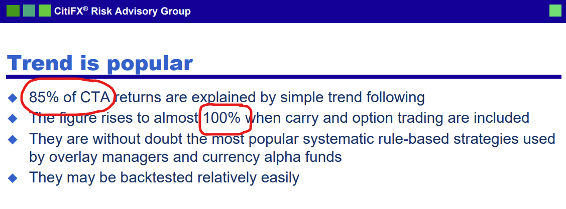
Follow the trend

• A classical example of a trending strategy uses the following system to describe the evolution of inflation \((\pi_t)\) and inflation expectations \((\pi^e_t)\) over time:
  
  

\[\pi^e_{t+2} = \alpha\pi_{t+1} + \xi(\pi_{t+1}-\pi_t) \tag{1}\]

\[\pi_{t+2} = \mu \pi^e_{t+2} \tag{2}\]

where \(\{\alpha , \xi, \mu\}\) are parameters.

• Inserting (2) into (1) we get:

\[\pi_{t+2} = \mu (\alpha\pi_{t+1} + \xi(\pi_{t+1}-\pi_t)) \tag{3}\]

• If, for simplicity, we assume \(\mu=\alpha=1\), we get:

\[\pi_{t+2} = \pi_{t+1} + \xi(\pi_{t+1}-\pi_t) \tag{4}\]

---

Follow the trend (cont,)

• Eq. (4) is a linear difference equation of second order with constant coefficients. Let’s add a random shock to it:
  
  

\[\pi_{t+2} = \pi_{t+1} +\underbrace{\xi(\pi_{t+1}-\pi_t)}_{\text{trend}} + \underbrace{\varepsilon_{t+2}}_{\text{random}} \tag{4a}\]

• Some immediate results can be figured out (ignore the random part for now):
  • If \(\pi_{t+1}=\pi_t\), then \(\pi_{t+2} = \pi_{t+1}\): inflation is stable
  • If \(\pi_{t+1}>\pi_t\), then \(\pi_{t+2} > \pi_{t+1}\): inflation is increasing
  • If \(\pi_{t+1}<\pi_t\), then \(\pi_{t+2} < \pi_{t+1}\): inflation is decreasing
  • If \(\pi_{t+1}=\pi_t\), and if \(\varepsilon_{t+2}>0\): inflation will be increasing
  • If \(\pi_{t+1}=\pi_t\), and if \(\varepsilon_{t+2}<0\): inflation will be decreasing

---

Create a new Pluto notebook from scratch

• Start Julia and run Pluto
• In the Pluto window click on the box Create a new notebook
• A new window will open with an empty notebook
• Save the new notebook:
  • Choose a folder on your computer to save the notebook
  • Add a notebook’s name at the end of the Path (e.g. 
    • \Desktop\M8674\Notebooks\Follow_the_Trend.jl
• Click on Choose to save the notebook
• The new notebook is ready to be used

---

Add some useful functionalities to the notebook

• When you start a new notebook, it looks like an empty box
• Add some packages:
  • Copy the code below and paste it into a new code cell
  • Run the cell: Shift + Enter or use the “Run” button

  begin
    using PlutoUI, Dates, SparseArrays , StatsBase, PlutoPlotly, PlotlyKaleido
    using CSV ,  DataFrames, LinearAlgebra , TimeSeries, NLsolve, LaTeXStrings
    force_pluto_mathjax_local(true)
    PlotlyKaleido.start(;mathjax = true)
  end

• Add a Table of Contents: copy the code below to a new cell and run it

TableOfContents() 

---

More Pluto functionalities

• The default width of the notebook is not very convenient for what we do:
  • Copy the code below and paste it into a new code cell
  • Run the cell: Shift + Enter or use the “Run” button

html"""
<style>
    @media screen {
        main {
            margin: 0 auto;
            max-width: 1600px;
            padding-left: max(200px, 10%);
            padding-right: max(383px, 10%);
            # 383px to accommodate TableOfContents(aside=true)
        }
    }
</style>
""" 

---

Final touch in the notebook

• Add a title to the notebook:

  • open a new cell and turn it into a Markdown cell

    • Ctrl + M then Enter

  • use the # symbol to create title sections, and subsections:

    • # for the main title
    • ## for a subtitle
    • ### for a sub-subtitle
    • …

  • Run the cell: Shift + Enter or use the “Run” button

  • Add your name, date, etc. using the same procedure in the notebook

---

Simulation: “Following the Trend” model

• Our model is given by eq. (3)

\[\pi_{t+2} = \mu (\alpha\pi_{t+1} + \xi(\pi_{t+1}-\pi_t)) \tag{3a}\]

• The easiest way to simulate this equation is to use a for loop.
• Consider the following baseline version:
  • Parameters: \(\mu = 1.0\) , \(\alpha = 1.0\) , \(\xi = 0.5\)
  • Iterations: \(n = 49\)
  • Initial conditions: \(\pi_1 = 2.0\) and \(\pi_2 = 2.0\)
  • Shock at \(t=20\): \(\epsilon_{20} = -0.5\)
• The code is given next.

---

Simulation

• Copy the code below, line by line, into a new cell, and run it

begin                                                   
    n = 49                  # Number of iterations
    μ = 1.0                     # Parameter: μ value
    α = 1.0                 # Parameter: α value
    ξ = 0.75                # Parameter: ξ value
    π_1 = [ 2.0  2.0 ]          # Setting the initial conditions (π₁=2.0, π₂=2.0)
    #l = length(π_1)            # Not very useful in simple models
    ϵ = zeros(1 , n+1)          # Defining the shocks, ϵ = zeros(l-1 , n+1) is an alternative
    ϵ[20] = 0.5                 # Inserting the only shock at t=20
    π = [π_1  zeros(1, n-1)]        # Pre-allocating space; alternative is π = [π_1  zeros(l-1, n-1)]
    
    for t = 1 : n-1
        π[t+2] = μ * (α * π[t+1] + ξ * (π[t+1] - π[t]) + ϵ[t+2])      # the equation to be iterated
    end
end

• Plot the results: copy the code below into a new cell and run it.

plot(π', mode = "markers+lines", line_width = 0.4)

---

5. Exponential smoothing

---

Exponential smoothing works for you

• Exponential smoothing gives more weight to recent data than to old data.
  • Uses also a simple rule of thumb to forecast the future.
  • Extrapolates also from what we have observed in in the past.
• A classical process that obeys exponential smoothing is given by:
  
  

\[P_{t}^{e}=P_{t-1}^{e}+\alpha\left(P_{t-1}-P_{t-1}^{e}\right) \ , \quad 0 \leq\alpha \leq1 \tag{5}\]

• \(P\) stands for the price level; \(P^e_t\) for the expected price level
• The parameter \(\alpha\) gives the velocity with which agents correct past mistakes:
  • \(\alpha \rightarrow 0\) ; past mistakes slowly corrected
  • \(\alpha \rightarrow 1\) ; past mistakes quickly corrected

---

The two classical papers

• Eq. (5) is the classical example of adaptive expectations
• The two seminal papers are: >Cagan, Philip (1956). The Monetary Dynamics of Hyperinflation. In Studies in the Quantity Theory of Money, ed. Milton Friedman, 25-117, University of Chicago Press.

Friedman, Milton (1957). A Theory of the Consumption Function. Princeton University Press.

• Cagan’s paper is about money demand & hyperinflation (Germany, 1920s)
• Friedman’s paper is about the consumption function

---

A Solution to eq. (5)

• Start with the eq. (5) above: \[P_{t}^{e}=P_{t-1}^{e}+\alpha\left(P_{t-1}-P_{t-1}^{e}\right) \tag{5a}\]

• Isolate \(P_{t-1}\) and get: \[P_{t}^{e}=\alpha P_{t-1}+(1-\alpha) P_{t-1}^{e} \tag{6}\]

• Iterate eq. (6) backward \(n\)-times, and the solution will be given by: (Jump to Appendix A for the derivation): \[P_{t}^{e}={\color{blue}(1-\alpha)^{n} P_{t-n}^{e}}+\sum_{i=0}^{n-1} \alpha(1-\alpha)^{i} P_{t-1-i} \tag{7}\]

---

\[P_{t}^{e}={\color{blue}(1-\alpha)^{n} P_{t-n}^{e}}+\sum_{i=0}^{n-1} \alpha(1-\alpha)^{i} P_{t-1-i} \tag{7a}\]

• To secure a stable solution in eq. (7a) we have to impose:
  \[|1-\alpha|<1\]

• If we assume \(0<\alpha<1\), the blue term above will converge to zero
  \[\lim _{n \rightarrow \infty}{\color{blue}(1-\alpha)^{n} P_{t-n}^{e}}=0\]

• And the stable solution will be:
  \[P_{t}^{e}=\sum_{i=0}^{n-1} \alpha(1-\alpha)^{i} P_{t-1-i} \tag{8}\]

• Main message: expected price level depends on past price levels through an exponential smoothing process.

---

6. Limitations of Adaptive Expectations

---

Adaptive expectations: good points & bad points

• The rules of thumb associated with AE seems to have some positive points:
  • They look like common sense rules (don’t repeat the same mistakes of the past)
  • They are easy to apply: collect data on some previous observations and make some simple calculations
  • And they are widely used in practice: algorithmic trading
• However, AE suffer from some serious drawbacks:
  • They are not logical: why should we use information only about the past? Why not information about what we expect that might happen in the future?
  • They can produce biased expectations: it leads to systematic mistakes
• See next figures.

---

Example 1: Exponential smoothing & the price level

width:780px

Consider a lag of 5 periods (quarters) and fast correction \(\alpha=0.95.\)

Looks great?

---

\(~\)

No, it looks quite poor.

The error in the forecasting exercise is large and systematic.

---

Example 2: Exponential smoothing & inflation rate

\(~\)

Let’s see what happens in the case of a stationary variable (inflation rate).

---

\(~\)

The vindication of Adaptive Expectations!

The mean of the mistakes is zero: \(-0.0094989\)!!

---

7. Stability: Predetermined (or backward-looking) variables

---

Predetermined (or backward-looking) variables

• A process is called predetermined if its deterministic part depends only upon past observations:
  \[x_{t+1}=\phi + \rho x_{t}+\varepsilon_{t+1} \ , \quad \varepsilon \sim \cal{N}(0,\sigma^2)\]

• Its dynamics will be expressed at the \(n\)-th iteration by: (jump to Appendix B for details) \[x_{t} = \color{teal} \sum_{i=0}^{n-1} \rho^{i} \phi+ \color{blue}\rho^{n} x_{t-n}+ \color{red}\sum_{i=0}^{n-1} \rho^{i} \varepsilon_{t-i} \tag{9}\]

• If \(|\rho|<1 :\) stable solution If \(|\rho|>1 :\) no stable solution If \(|\rho|=1 :\) no solution

---

Predetermined variables: stable solution

• By imposing the condition \(|\rho|<1\), eq. (9) will be written as:

\[x_{t} = \color{teal} \sum_{i=0}^{n-1} \rho^{i} \phi+ \color{red}\sum_{i=0}^{n-1} \rho^{i} \varepsilon_{t-i} \tag{9a}\]

• Applying the formula for the sum of a geometric series, (9a) can be simplified as:

\[x_{t} = \frac{\phi}{1-\rho} + \sum_{i=0}^{n-1} \rho^{i} \varepsilon_{t-i} \tag{10}\]

• If there were no shocks in the past, the solution will correspond to the deterministic steady state of the original process:

\[x_{t} = \overline{x} =\frac{\phi}{1-\rho} \tag{11}\]

---

8. Readings

---

• There is no compulsory reading for this session. We hope that the slides and the notebook will be sufficient to provide a good grasp of the adaptive expectations approach in macroeconomics.
• Many textbooks deal with this subject in a way that is not very useful for our course. They treat this subject in an elementary way or offer a very sophisticated presentation, usually extremely mathematical but short on content.
• There is a textbook that feels quite good for our level: Patrick Minford and David Peel (2019). Advanced Macroeconomics: Primer, Second Edition, Edward Elgar, Cheltenham.
• Chapter 2 deals extensively with adaptive and rational expectations. However, this chapter is quite long (40 pages), making it more suitable to be used as complementary material rather than as compulsory reading. But it is by far the best treatment of this subject at this level.

---

• Another excellent treatment of adaptive expectations can be found in the textbook:

  Ben J. Heijdra (2017). Foundations of Modern Macroeconomics. Third Edition, Oxford UP, Oxford.

  • Chapter 5 deal with this topic at great length (40 pages), but the subject is discussed at a relatively more advanced level than the one we follow in our course.

• Another source of information is the book by:

  • George W. Evans and Seppo Honkapohja (2009). Learning and Expectations in Macroeconomics, Second Edition, Princeton UP, Princeton.
  • Chapter 1 (Expectations and the learning approach) deals with this topic at an elementary level, because their idea is to focus on what they call “learning”.

---

Appendix A

A step-by-step derivation of equation (7) in the next slides

Jump back to eq. (5)

---

Solution: backward iteration

• We will solve the following equation by backward iteration: \[P_{t}^{e}=\alpha P_{t-1}+(1-\alpha) P_{t-1}^{e}\]

• Like this, when \(n \rightarrow \infty\): \[\underbrace{t \rightarrow (t-1)}_{1\text{st iteration}} \rightarrow \underbrace{(t-1) \rightarrow (t-2)}_{2\text{nd iteration}} \rightarrow \underbrace{(t-2) \rightarrow (t-3)}_{3\text{rd iteration}} \rightarrow ... \rightarrow\underbrace{(t-(n-1)) \rightarrow (t-n)}_{n\text{th iteration}}\]

• The strategy is as follows:

  • Iterate up to the 3rd iteration: see a pattern at this iteration
  • Then, generalize to the \(n\)th iteration

---

Let’s start: 1st iteration

\(P_{t}^{e}=\alpha P_{t-1}+(1-\alpha) P_{t-1}^{e} \qquad \qquad \qquad \qquad \qquad \qquad \ \ \qquad\) 1st iteration: t \(\rightarrow\) t-1

---

Going 1 period backward

\(P_{t}^{e}=\alpha P_{t-1}+(1-\alpha) P_{t-1}^{e} \qquad \qquad \qquad \qquad \qquad \qquad \ \ \qquad\) 1st iteration: t \(\rightarrow\) t-1

\(\color{gray} \downarrow \qquad \qquad \qquad \qquad \qquad \ \nwarrow P_{t-1}^{e}=\alpha P_{t-2}+(1-\alpha) P_{t-2}^{e} \qquad \qquad\) back 1 period

---

Get the result in the 2nd iteration

\(P_{t}^{e}=\alpha P_{t-1}+(1-\alpha) P_{t-1}^{e} \qquad \qquad \qquad \qquad \qquad \qquad \ \ \qquad\) 1st iteration: t \(\rightarrow\) t-1

\(\color{gray} \downarrow \qquad \qquad \qquad \qquad \qquad \ \nwarrow P_{t-1}^{e}=\alpha P_{t-2}+(1-\alpha) P_{t-2}^{e} \qquad \qquad\) back 1 period

\(P_{t}^{e}=\alpha P_{t-1}+(1-\alpha)\left[\alpha P_{t-2}+(1-\alpha) P_{t-2}^{e}\right]\qquad \quad \qquad~\) 2nd iteration: t-1 \(\rightarrow\) t-2

---

Simplify the result in the 2nd iteration

\(P_{t}^{e}=\alpha P_{t-1}+(1-\alpha) P_{t-1}^{e} \qquad \qquad \qquad \qquad \qquad \qquad \ \ \qquad\) 1st iteration: t \(\rightarrow\) t-1

\(\color{gray} \downarrow \qquad \qquad \qquad \qquad \qquad \ \nwarrow P_{t-1}^{e}=\alpha P_{t-2}+(1-\alpha) P_{t-2}^{e} \qquad \qquad\) back 1 period

\(P_{t}^{e}=\alpha P_{t-1}+(1-\alpha)\left[\alpha P_{t-2}+(1-\alpha) P_{t-2}^{e}\right]\)

\(P_{t}^{e}=\alpha P_{t-1}+\alpha (1-\alpha) P_{t-2}+(1-\alpha)^{2} P_{t-2}^{e} \qquad \qquad \qquad\) 2nd iteration: t-1 \(\rightarrow\) t-2

---

Going 2 periods backward

\(P_{t}^{e}=\alpha P_{t-1}+(1-\alpha) P_{t-1}^{e} \qquad \qquad \qquad \qquad \qquad \qquad \ \ \qquad\) 1st iteration: t \(\rightarrow\) t-1

\(\color{gray} \downarrow \qquad \qquad \qquad \qquad \qquad \ \nwarrow P_{t-1}^{e}=\alpha P_{t-2}+(1-\alpha) P_{t-2}^{e} \qquad \qquad\) back 1 period

\(P_{t}^{e}=\alpha P_{t-1}+(1-\alpha)\left[\alpha P_{t-2}+(1-\alpha) P_{t-2}^{e}\right]\)

\(P_{t}^{e}=\alpha P_{t-1}+\alpha (1-\alpha) P_{t-2}+(1-\alpha)^{2} P_{t-2}^{e} \qquad \qquad \qquad\) 2nd iteration: t-1 \(\rightarrow\) t-2

\(\color{gray} \downarrow \qquad \qquad \qquad \qquad \qquad \qquad \qquad \qquad \qquad \nwarrow P_{t-2}^{e}=\alpha P_{t-3}+(1-\alpha) P_{t-3}^{e}\)

---

Get the result in the 3rd iteration

\(P_{t}^{e}=\alpha P_{t-1}+(1-\alpha) P_{t-1}^{e} \qquad \qquad \qquad \qquad \qquad \qquad \ \ \qquad\) 1st iteration: t \(\rightarrow\) t-1

\(\color{gray} \downarrow \qquad \qquad \qquad \qquad \qquad \ \nwarrow P_{t-1}^{e}=\alpha P_{t-2}+(1-\alpha) P_{t-2}^{e} \qquad \qquad\) back 1 period

\(P_{t}^{e}=\alpha P_{t-1}+(1-\alpha)\left[\alpha P_{t-2}+(1-\alpha) P_{t-2}^{e}\right]\)

\(P_{t}^{e}=\alpha P_{t-1}+\alpha (1-\alpha) P_{t-2}+(1-\alpha)^{2} P_{t-2}^{e} \qquad \qquad \qquad\) 2nd iteration: t-1 \(\rightarrow\) t-2

\(\color{gray} \downarrow \qquad \qquad \qquad \qquad \qquad \qquad \qquad \qquad \qquad \nwarrow P_{t-2}^{e}=\alpha P_{t-3}+(1-\alpha) P_{t-3}^{e}\)

\(P_{t}^{e}=\alpha P_{t-1}+ \alpha (1-\alpha) P_{t-2}+(1-\alpha)^{2}\left[\alpha P_{t-3}+(1-\alpha) P_{t-3}^{e}\right]\)

\(P_{t}^{e} = \alpha P_{t-1}+ \alpha (1-\alpha) P_{t-2}+\alpha (1-\alpha)^{2} P_{t-3}+\color{blue}{(1-\alpha)^{3} P_{t-3}^{e}}~~~\) 3rd iter.: t-2 \(\rightarrow\) t-3

---

Simplify the result in the 3rd iteration

\(P_{t}^{e}=\alpha P_{t-1}+(1-\alpha) P_{t-1}^{e} \qquad \qquad \qquad \qquad \qquad \qquad \ \ \qquad\) 1st iteration: t \(\rightarrow\) t-1

\(\color{gray} \downarrow \qquad \qquad \qquad \qquad \qquad \ \nwarrow P_{t-1}^{e}=\alpha P_{t-2}+(1-\alpha) P_{t-2}^{e} \qquad \qquad\) back 1 period

\(P_{t}^{e}=\alpha P_{t-1}+(1-\alpha)\left[\alpha P_{t-2}+(1-\alpha) P_{t-2}^{e}\right]\)

\(P_{t}^{e}=\alpha P_{t-1}+\alpha (1-\alpha) P_{t-2}+(1-\alpha)^{2} P_{t-2}^{e} \qquad \qquad \qquad\) 2nd iteration: t-1 \(\rightarrow\) t-2

\(\color{gray} \downarrow \qquad \qquad \qquad \qquad \qquad \qquad \qquad \qquad \qquad \nwarrow P_{t-2}^{e}=\alpha P_{t-3}+(1-\alpha) P_{t-3}^{e}\)

\(P_{t}^{e}=\alpha P_{t-1}+ \alpha (1-\alpha) P_{t-2}+(1-\alpha)^{2}\left[\alpha P_{t-3}+(1-\alpha) P_{t-3}^{e}\right]\)

\(P_{t}^{e} = \alpha P_{t-1}+ \alpha (1-\alpha) P_{t-2}+\alpha (1-\alpha)^{2} P_{t-3}+\color{blue}{(1-\alpha)^{3} P_{t-3}^{e}}~~~\) 3rd iter.: t-2 \(\rightarrow\) t-3

\[P_{t}^{e}=\sum_{i=0}^{3-1} \alpha(1-\alpha)^{i} P_{t-1-i}+{\color{blue}(1-\alpha)^{3} P_{t-3}^{e}}\]

---

Generalize to the \(n\)-th iteration

• In the previous slide, we iterated backwards 3 times.

• The result was: \[P_{t}^{e}=\sum_{i=0}^{3-1} \alpha(1-\alpha)^{i} P_{t-1-i}+{\color{blue}(1-\alpha)^{3} P_{t-3}^{e}}\]

• Now, it is easy to see that if we iterate \(n\)-times backward, instead of 3, we will get:

\[P_{t}^{e}=\sum_{i=0}^{n-1} \alpha(1-\alpha)^{i} P_{t-1-i}+{\color{blue}(1-\alpha)^{n} P_{t-n}^{e}}\]

Jump back to eq. (5)

---

Appendix B

Students are advised to read this slide carefully.

A step-by-step derivation of equation (9) in the following slides

Jump back to eq. (9)

---

Solution: backward iteration

• We will solve the following equation by backward iteration: \[x_{t}=\phi+\rho x_{t-1}+\varepsilon_{t}\]

• Like this, when \(n \rightarrow \infty\): \[\underbrace{t \rightarrow (t-1)}_{1\text{st iteration}} \rightarrow \underbrace{(t-1) \rightarrow (t-2)}_{2\text{nd iteration}} \rightarrow \underbrace{(t-2) \rightarrow (t-3)}_{3\text{rd iteration}} \rightarrow ... \rightarrow\underbrace{(t-(n-1)) \rightarrow (t-n)}_{n\text{th iteration}}\]

• The strategy is as follows:

  • Iterate up to the 3rd iteration: see a pattern at this iteration
  • Then, generalize to the \(n\)th iteration

---

Let us start: 1st iteration

\(x_{t}=\phi+\rho x_{t-1}+\varepsilon_{t} \qquad \qquad \qquad \qquad \qquad \qquad \qquad\) 1st iteration: \(\ t \rightarrow t-1\)

---

Going 1 period back in time

\(x_{t}=\phi+\rho x_{t-1}+\varepsilon_{t} \qquad \qquad \qquad \qquad \qquad \qquad \qquad\) 1st iteration: \(\ t \rightarrow t-1\)

\(\color{gray} \downarrow \qquad \qquad \qquad \nwarrow x_{t-1}=\phi+\rho x_{t-2}+\varepsilon_{t-1} \ \ \qquad \quad \qquad\) going back 1 period

---

Let’s get the result in the 2nd iteration

\(x_{t}=\phi+\rho x_{t-1}+\varepsilon_{t} \qquad \qquad \qquad \qquad \qquad \qquad \qquad\) 1st iteration: \(\ t \rightarrow t-1\)

\(\color{gray} \downarrow \qquad \qquad \qquad \nwarrow x_{t-1}=\phi+\rho x_{t-2}+\varepsilon_{t-1} \ \ \qquad \quad \qquad\) going back 1 period

\(x_{t}=\phi+\rho\left[\phi+\rho x_{t-2}+\varepsilon_{t-1}\right]+\varepsilon_{t}\)

---

Simplify the result in the 2nd iteration

\(x_{t}=\phi+\rho x_{t-1}+\varepsilon_{t} \qquad \qquad \qquad \qquad \qquad \qquad \qquad\) 1st iteration: \(\ t \rightarrow t-1\)

\(\color{gray} \downarrow \qquad \qquad \qquad \nwarrow x_{t-1}=\phi+\rho x_{t-2}+\varepsilon_{t-1} \ \ \qquad \quad \qquad\) going back 1 period

\(x_{t}=\phi+\rho\left[\phi+\rho x_{t-2}+\varepsilon_{t-1}\right]+\varepsilon_{t}\)

\(x_t=\phi+\rho \phi+\rho^{2} x_{t-2}+\rho \varepsilon_{t-1}+\varepsilon_{t} \ \ \ \qquad \quad \qquad\) 2nd iteration: \(\ t-1 \rightarrow t-2\)

---

Going 2 periods back in time

\(x_{t}=\phi+\rho x_{t-1}+\varepsilon_{t} \qquad \qquad \qquad \qquad \qquad \qquad \qquad\) 1st iteration: \(\ t \rightarrow t-1\)

\(\color{gray} \downarrow \qquad \qquad \qquad \nwarrow x_{t-1}=\phi+\rho x_{t-2}+\varepsilon_{t-1} \ \ \qquad \quad \qquad\) going back 1 period

\(x_{t}=\phi+\rho\left[\phi+\rho x_{t-2}+\varepsilon_{t-1}\right]+\varepsilon_{t}\)

\(x_t=\phi+\rho \phi+\rho^{2} x_{t-2}+\rho \varepsilon_{t-1}+\varepsilon_{t} \ \ \ \qquad \quad \qquad\) 2nd iteration: \(\ t-1 \rightarrow t-2\)

\(\color{gray} \downarrow \qquad \qquad \qquad \qquad \ \nwarrow x_{t-2}=\phi+\rho x_{t-3}+\varepsilon_{t-2} \ \qquad\) going back 2 periods

---

Let’s get the result in the 3rd iteration

\(x_{t}=\phi+\rho x_{t-1}+\varepsilon_{t} \qquad \qquad \qquad \qquad \qquad \qquad \qquad\) 1st iteration: \(\ t \rightarrow t-1\)

\(\color{gray} \downarrow \qquad \qquad \qquad \nwarrow x_{t-1}=\phi+\rho x_{t-2}+\varepsilon_{t-1} \ \ \qquad \quad \qquad\) going back 1 period

\(x_{t}=\phi+\rho\left[\phi+\rho x_{t-2}+\varepsilon_{t-1}\right]+\varepsilon_{t}\)

\(x_t=\phi+\rho \phi+\rho^{2} x_{t-2}+\rho \varepsilon_{t-1}+\varepsilon_{t} \ \ \ \qquad \quad \qquad\) 2nd iteration: \(\ t-1 \rightarrow t-2\)

\(\color{gray} \downarrow \qquad \qquad \qquad \qquad \ \nwarrow x_{t-2}=\phi+\rho x_{t-3}+\varepsilon_{t-2} \ \qquad\) going back 2 periods

\(x_{t} = \color{teal} \quad \phi+\rho \phi+\rho^{2} \phi+\color{blue} \rho^{3} x_{t-3}+ \color{red}\rho^{2} \varepsilon_{t-2}+\rho^{1} \varepsilon_{t-1}+ \ \ \varepsilon_{t}\color{black}\) \(x_{t} =\color{teal}\rho^0 \phi+\rho^{1} \phi+\rho^{2} \phi+\color{blue} \rho^{3} x_{t-3}+ \color{red}\rho^{2} \varepsilon_{t-2}+\rho^{1} \varepsilon_{t-1}+\rho^{0} \varepsilon_{t}\color{black}\)

---

Simplify the result in the 3rd iteration

\(x_{t}=\phi+\rho x_{t-1}+\varepsilon_{t} \qquad \qquad \qquad \qquad \qquad \qquad \qquad\) 1st iteration: \(\ t \rightarrow t-1\)

\(\color{gray} \downarrow \qquad \qquad \qquad \nwarrow x_{t-1}=\phi+\rho x_{t-2}+\varepsilon_{t-1} \ \ \qquad \quad \qquad\) going back 1 period

\(x_{t}=\phi+\rho\left[\phi+\rho x_{t-2}+\varepsilon_{t-1}\right]+\varepsilon_{t}\)

\(x_t=\phi+\rho \phi+\rho^{2} x_{t-2}+\rho \varepsilon_{t-1}+\varepsilon_{t} \ \ \ \qquad \quad \qquad\) 2nd iteration: \(\ t-1 \rightarrow t-2\)

\(\color{gray} \downarrow \qquad \qquad \qquad \qquad \ \nwarrow x_{t-2}=\phi+\rho x_{t-3}+\varepsilon_{t-2} \ \qquad\) going back 2 periods

\(x_{t} = \color{teal} \quad \phi+\rho \phi+\rho^{2} \phi+\color{blue} \rho^{3} x_{t-3}+ \color{red}\rho^{2} \varepsilon_{t-2}+\rho^{1} \varepsilon_{t-1}+ \ \ \varepsilon_{t}\color{black}\)

\(x_{t} =\color{teal}\rho^0 \phi+\rho^{1} \phi+\rho^{2} \phi+\color{blue} \rho^{3} x_{t-3}+ \color{red}\rho^{2} \varepsilon_{t-2}+\rho^{1} \varepsilon_{t-1}+\rho^{0} \varepsilon_{t}\color{black}\)

\[x_{t} = \color{teal} \sum_{i=0}^{3-1} \rho^{i} \phi+ \color{blue}\rho^{3} x_{t-3}+ \color{red}\sum_{i=0}^{3-1} \rho^{i} \varepsilon_{t-i} \color{black} \qquad \qquad \qquad \qquad \text{$3$rd iteration:} \ t-2 \rightarrow t-3\]

---

Generalize to the \(n\)-th iteration

• In the previous slide, we iterated backwards 3 times.

• The result was:

\[x_{t} = \color{teal} \sum_{i=0}^{3-1} \rho^{i} \phi+ \color{blue}\rho^{3} x_{t-3}+ \color{red}\sum_{i=0}^{3-1} \rho^{i} \varepsilon_{t-i}\]

• Now, it is easy to see that if we iterate \(n\)-times, instead of 3, we will get:

\[x_{t} = \color{teal} \sum_{i=0}^{n-1} \rho^{i} \phi+ \color{blue}\rho^{n} x_{t-n}+ \color{red}\sum_{i=0}^{n-1} \rho^{i} \varepsilon_{t-i}\]

Back to eq. (9)