---

marp: true author: Vivaldo Mendes paginate: true style: | .columns { display: grid; grid-template-columns: minmax(0, 50fr) minmax(0, 50fr); } h2 { position: absolute; top: 50px; left: 75px; right: 75px; color: #34429a; font-size: 46px; }

h1 { font-size: 60px }

---

Filters & Impulse Response Functions

Macroeconomics (M8674), March 2025

Vivaldo Mendes, ISCTE

vivaldo.mendes@iscte-iul.pt

---

1. Filters

---

Types of Filters

• Main objective: to separate the long-run trend from the short-run cyclical component of a time series $y(t)$ .
• There are various approaches to achieve this:
  • Linear filter
  • Linear filter with breaks
  • Nonlinear filters
• Nonlinear filters
  • Hodrick-Prescott filter (Hodrick & Prescott, 1997)
  • Band Pass filter (Baxter & King, 1999)
  • Hamilton filter (James Hamilton, 2017)
  • … and some others

---

The Hodrick-Prescott filter (HP)

• The HP filter is the most used filter in macroeconomics

• It is given by the minimization problem:
  

  $$\begin{array}{}\text{(1)}& \underset{{\tau }_t}{min}\sum _{t=1}^T\{{(y_t-{\tau }_t)}^2+\lambda {[({\tau }_{t+1}-{\tau }_t)-({\tau }_t-{\tau }_{t-1})]}^2\}\end{array}$$

• where:

  • $y_t$ is the observed time series
  • ${\tau }_t$ is the smooth trend that we want to obtain
  • $\lambda$ is the parameter that we set to obtain the desired smoothness in the trend

---

The HP filter: Special Cases

The value given to parameter $\lambda$ is a choice of ours:

$$\underset{{\tau }_t}{min}\sum _{t=1}^T\{{(y_t-{\tau }_t)}^2+\lambda {[({\tau }_{t+1}-{\tau }_t)-({\tau }_t-{\tau }_{t-1})]}^2\}$$

• $\lambda =0$ $\Rightarrow$ trivial solution because there are no cycles : $y_t={\tau }_t,\mathrm{\forall }t$
• $\lambda \to \mathrm{\infty }\Rightarrow$ linear trend leads to huge cycles between $y_t$ and ${\tau }_t$
• $\lambda =1600$ $\Rightarrow$ duration/amplitude of cycles acceptable for quarterly data
• $\lambda =7$ $\Rightarrow$ duration/amplitude of cycles acceptable for annual data
• There is no “unquestionable” value for $\lambda$

---

The HP Filter: an Example

• Main objective: obtain cycles as % deviations from the trend
• This has an important implication:
  • Time series with a trend: apply logs to the data before extracting the trend and the cycles
  • Time series without a clear trend: do not apply logs to the data
• Quarterly data: “US_data.csv”
• A simple example:
  • Real GDP (GDP)
  • Consumer Price Index (CPI)
  • Unemployment Rate (UR)

---

width:1200px

---

Dealing with rows and columns in a Matrix

$$

---

Compute the HP filter: a single variable

$$

---

Compute the HP filter: a single variable (another way)

$$

---

Compute the HP filter: several variables

$$

---

Compute the business-cycles: several variables

$$

---

Business cycles: Inflation and Unemployment

$$The inflation-gap $$The unemployment-gap

---

The output-gap: logs vs levels

$$ Correctly measured: using logs $$Incorrectly measured: using levels

---

2. Impulse Response Functions

---

What are IRFs?

• Impulse response functions represent the response of the endogenous variables of a given system, when one (or more than one) of its endogenous variables is hit by an exogenous shock.
• The nature of the shock can be:
  • Temporary
  • Permanent
  • Systematic
• Linear systems. The magnitude of the shock does not change the stability properties of the system.
• Nonlinear systems. In this case, the magnitude of the shock is of great inportance and it can change the stability of the system under consideration.

---

An example

• Consider the simplest case, an AR(1):

$$\begin{array}{}\text{(2)}& y_{t+1}=a{y}_t+{\epsilon }_{t+1},{\epsilon }_t\sim N(0,1)\end{array}$$

• Assume that for $t\in (1,n)$: $$y_1=0;{\epsilon }_2=1;{\epsilon }_t=0,\mathrm{\forall }t\ne 2$$
• This implies that at $t=2\Rightarrow y_2=1$. But what happens next, if there are no more shocks?
• The IRF of $y$ provides the answer.
• The dynamics of $y$ will depend crucially on the value of $a$. Six examples: $$a=\{0,0.5,0.9,0.99,1,1.01\}$$

---

The IRFs of the AR(1) Process

$$

---

Another example

• Consider a more sophisticated case, an AR(2):

$$y_{t+1}=a{y}_t+b{y}_{t-1}+{\epsilon }_{t+1},{\epsilon }_t\sim N(0,1)$$ * Assume that for $t\in (1,n)$: $$y_1=0;y_2=0;{\epsilon }_3=1;{\epsilon }_t=0,\mathrm{\forall }t\ne 3$$

• This implies that at
  $$t=3,{\epsilon }_3=1\Rightarrow y_3=1.$$

• What happens next, if there are no more shocks? The IRF of $y$ provides the answer.

• The dynamics of $y$ will depend on the values of $a$ and $b$. For simplicity consider: $$b=-0.9;a=\{1.85,1.895,1.9,1.9005\}$$

---

The IRFs of the AR(2) Process

$$

---

More Sophisticated Examples

• A similar reasoning can be applied to our rather more general model: $$\begin{array}{}\text{(3)}& X_{t+1}=A+B{X}_t+C{\epsilon }_{t+1}\end{array}$$

• .. where $B,C$ are $n\times n$ matrices, while $X_{t+1},X_t,A,{\epsilon }_{t+1}$ are $n\times 1$ vectors.

• Consider the following VAR(3) model: $$X_{t+1}=\left[\begin{array}{c}{z}_{t+1}\\ w_{t+1}\\ v_{t+1}\end{array}\right]$$

---

• In this example we take matrices $A,B$ and $C$ given by: $$

  $$\begin{array}{c}A=\left[\begin{array}{c}0.0\\ 0.0\\ 0.0\end{array}\right],B=\left[\begin{array}{rrr}0.97& 0.10& -0.05\\ -0.3& 0.8& 0.05\\ 0.01& -0.04& 0.96\end{array}\right],C=\left[\begin{array}{lll}1.0& 0.0& 0.0\\ 0.0& 0.0& 0.0\\ 0.0& 0.0& 0.0\end{array}\right].\end{array}$$

  $$

• The initial state of our system (or its initial conditions) are: $z_1=0,w_1=0$ and $v_1=0$, that is: $$X_1=[0,0,0]$$

• The shock only hits the variable $z_t$ $($notice the blue entry in matrix $C)$, and we assume that the shock occurs in period $t=3$.

• What happens to the dynamics of the three endogenous variables? See next figure.

---

The IRFs of our VAR(3) Process

$$

---

AR(1): A Sequence of Shocks

Consider the same AR(1) as in eq. (2). But now impose a sequence of 200 shocks.

$$

---

Implications of a Linear Structure

• In the previous examples, the structure of all our models was linear.
• This has a crucial implication: The shock’s magnitude did not alter the dynamics produced by the shock itself.
  • Only the structure of the model would lead to different outcomes.
• This does not usually occur if the structure of the model is non-linear. In this case, the magnitude of the shock may produce different outcomes even if the system’s structure remains the same.
• We do not have time to cover this particular point.
• But be careful: if the structure of the model is non-linear, large shocks can not be simulated … in a linearized version of the original system.

---

3. Important Problems

---

Three Major Issues

• There is no perfect filter … but the HP seems the best.
• Measuring Potential GDP (or Natural Unemployment) is difficult:
  • Potential GDP is usually associated with the HP-trend in GDP … but not exclusively.
  • The Natural Rate of Unemployment is largely associated with the HP-trend in unemployment.
• All macroeconomic models are non-linear:
  • Be careful with IRFs that are produced by a linearized version of the model.
  • Big shocks are difficult to be fully represented by linearization.

---

Limitations of the HP Filter

• New data leads to the rewriting of the history of the economy
• The HP filter is extremely useful but should be used with care

| | |

---

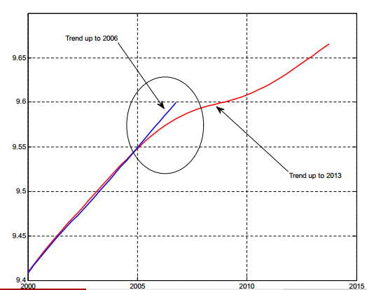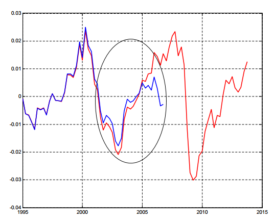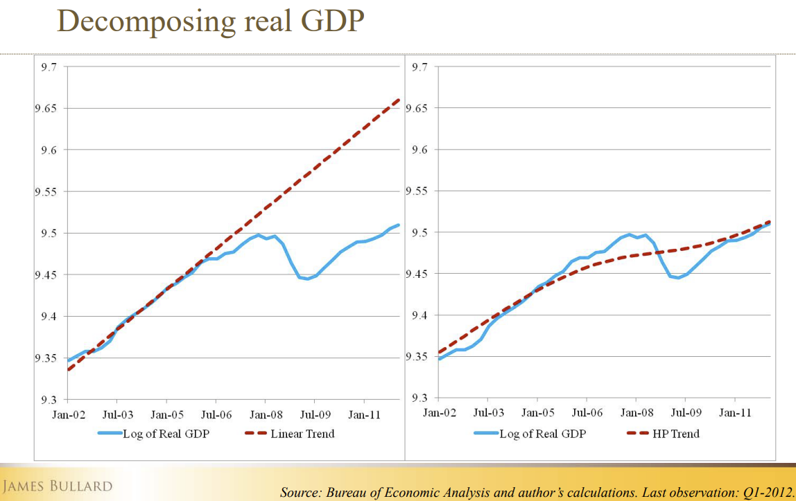
Misuses of the HP Filter

• In 2012, the US economy had an unemployment rate close to 8%, one of the highest rates since WWII.
• The Fed Funds Rate was at 0%, to stimulate the economy.
• The inflation rate was much below the target level (2%) at 0.5% and showing signs of going down.
• James Bullard (the President of the FRB of St. Louis), in a famous speech in June 2012 defended that the US economy had gone back to Potential GDP.
  • He defended that the Fed should produce a sharp increase in the Fed Funds Rate.
  • He used the HP-filter to substantiate his proposal.

---

The HP filter according to James Bullard

$$

---

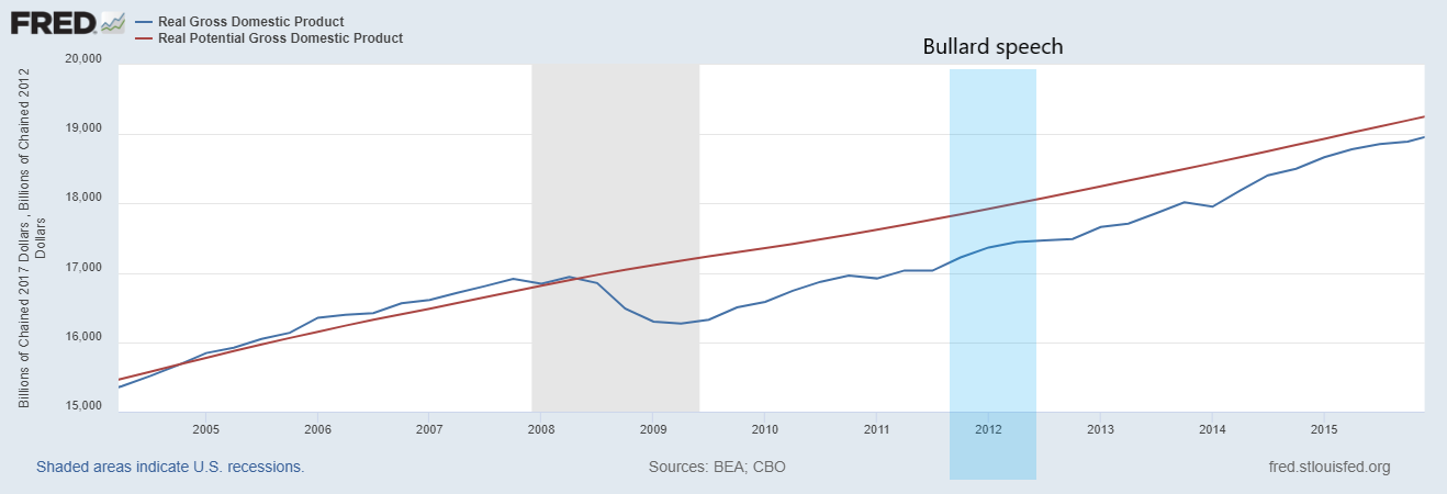
The Output-gap According to the FRB … St. Louis

The FRB of St. Louis publishes “oficial” US data for Real GDP and Potential GDP.

$$

---

The Natural Rate of Unemployment (NRU)

No, Covid-19 did not raise the NRU; no, an increase in NRU did not anticipate Covid-19!

$$

---

4. Readings

---

Point 1

• For this point, there is no compulsory reading.

• However, Dirk Krueger (2007). “Quantitative Macroeconomics: An Introduction” (Chapter 2), manuscript, Department of Economics University of Pennsylvania, is well suited for the material covered here.

• This text is a small one (12 pages), easy to read, and beneficial for studying the stylized facts of business cycles, mainly to understand how the Hodrick-Prescott filter is calculated. However, notice that, as mentioned, it is not compulsory reading.

---

Point 2

• For this point, there is no compulsory reading. However, any modern textbook on time series will cover this subject.
• At an introductory level, see sections 11.8 and 11.9 of the textbook: Diebold, F. X. (1998). Elements of forecasting. South-Western College Pub, Cincinnati.
• At a more advanced level, see, e.g., section 2.3.2 of the textbook: Lütkepohl, H. (2007). New introduction to multiple time series analysis (2nd ed.), Springer, Berlin.

---

Point 3

• No textbook covers the topics/controversies mentioned in this section.
• This coursework intends to provide a framework for a better understanding of these controversies at the end of the course.
• All we have to handle is:
  • A little bit of mathematics
  • A little bit of computation
  • A little bit of macroeconomics