Filters & Impulse Response Functions

Macroeconomics (M8674), March 2025

Vivaldo Mendes, ISCTE

vivaldo.mendes@iscte-iul.pt

1. Filters

Types of Filters

• Main objective: to separate the long-run trend from the short-run cyclical component of a time series .
• There are various approaches to achieve this:
  • Linear filter
  • Linear filter with breaks
  • Nonlinear filters
• Nonlinear filters
  • Hodrick-Prescott filter (Hodrick & Prescott, 1997)
  • Band Pass filter (Baxter & King, 1999)
  • Hamilton filter (James Hamilton, 2017)
  • ... and some others

The Hodrick-Prescott filter (HP)

• The HP filter is the most used filter in macroeconomics

• It is given by the minimization problem:
  
  

• where:

  • is the observed time series
  • is the smooth trend that we want to obtain
  • is the parameter that we set to obtain the desired smoothness in the trend

The HP filter: Special Cases

The value given to parameter is a choice of ours:

• trivial solution because there are no cycles :
• linear trend leads to huge cycles between and
• duration/amplitude of cycles acceptable for quarterly data
• duration/amplitude of cycles acceptable for annual data
• There is no "unquestionable" value for

The HP Filter: an Example

• Main objective: obtain cycles as % deviations from the trend
• This has an important implication:
  • Time series with a trend: apply logs to the data before extracting the trend and the cycles
  • Time series without a clear trend: do not apply logs to the data
• Quarterly data: "US_data.csv"
• A simple example:
  • Real GDP (GDP)
  • Consumer Price Index (CPI)
  • Unemployment Rate (UR)

Dealing with rows and columns in a Matrix

Compute the HP filter: a single variable

Compute the HP filter: a single variable (another way)

Compute the HP filter: several variables

Compute the business-cycles: several variables

Business cycles: Inflation and Unemployment

The inflation-gap The unemployment-gap

The output-gap: logs vs levels

Correctly measured: using logs Incorrectly measured: using levels

2. Impulse Response Functions

What are IRFs?

• Impulse response functions represent the response of the endogenous variables of a given system, when one (or more than one) of its endogenous variables is hit by an exogenous shock.
• The nature of the shock can be:
  • Temporary
  • Permanent
  • Systematic
• Linear systems. The magnitude of the shock does not change the stability properties of the system.
• Nonlinear systems. In this case, the magnitude of the shock is of great inportance and it can change the stability of the system under consideration.

An example

• Consider the simplest case, an AR(1):

• Assume that for :

• This implies that at . But what happens next, if there are no more shocks?
• The IRF of provides the answer.
• The dynamics of will depend crucially on the value of . Six examples:

The IRFs of the AR(1) Process

Another example

• Consider a more sophisticated case, an AR(2):

• Assume that for :

• This implies that at

• What happens next, if there are no more shocks? The IRF of provides the answer.

• The dynamics of will depend on the values of and . For simplicity consider:

The IRFs of the AR(2) Process

More Sophisticated Examples

• A similar reasoning can be applied to our rather more general model:

• .. where are matrices, while are vectors.

• Consider the following VAR(3) model:

• In this example we take matrices and given by:

• The initial state of our system (or its initial conditions) are: and , that is:

• The shock only hits the variable notice the blue entry in matrix , and we assume that the shock occurs in period .

• What happens to the dynamics of the three endogenous variables? See next figure.

The IRFs of our VAR(3) Process

AR(1): A Sequence of Shocks

Consider the same AR(1) as in eq. (2). But now impose a sequence of 200 shocks.

Implications of a Linear Structure

• In the previous examples, the structure of all our models was linear.
• This has a crucial implication:
  The shock's magnitude did not alter the dynamics produced by the shock itself.
  • Only the structure of the model would lead to different outcomes.
• This does not usually occur if the structure of the model is non-linear. In this case, the magnitude of the shock may produce different outcomes even if the system's structure remains the same.
• We do not have time to cover this particular point.
• But be careful: if the structure of the model is non-linear, large shocks can not be simulated ... in a linearized version of the original system.

3. Important Problems

Three Major Issues

• There is no perfect filter ... but the HP seems the best.
• Measuring Potential GDP (or Natural Unemployment) is difficult:
  • Potential GDP is usually associated with the HP-trend in GDP ... but not exclusively.
  • The Natural Rate of Unemployment is largely associated with the HP-trend in unemployment.
• All macroeconomic models are non-linear:
  • Be careful with IRFs that are produced by a linearized version of the model.
  • Big shocks are difficult to be fully represented by linearization.

Limitations of the HP Filter

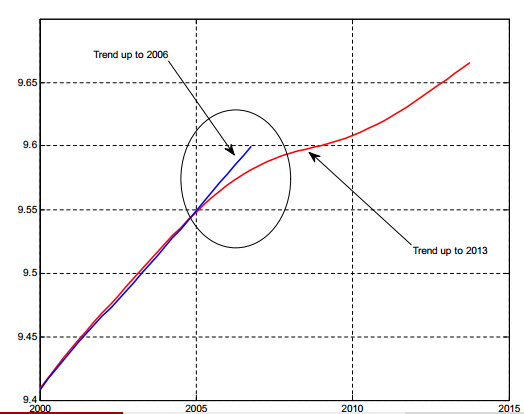
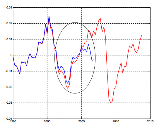
• New data leads to the rewriting of the history of the economy
• The HP filter is extremely useful but should be used with care

| | |

Misuses of the HP Filter

• In 2012, the US economy had an unemployment rate close to 8%, one of the highest rates since WWII.
• The Fed Funds Rate was at 0%, to stimulate the economy.
• The inflation rate was much below the target level (2%) at 0.5% and showing signs of going down.
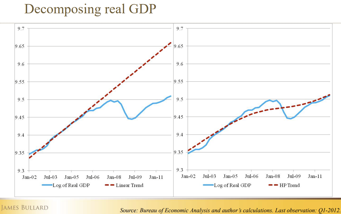
• James Bullard (the President of the FRB of St. Louis), in a famous speech in June 2012 defended that the US economy had gone back to Potential GDP.
  • He defended that the Fed should produce a sharp increase in the Fed Funds Rate.
  • He used the HP-filter to substantiate his proposal.

The HP filter according to James Bullard

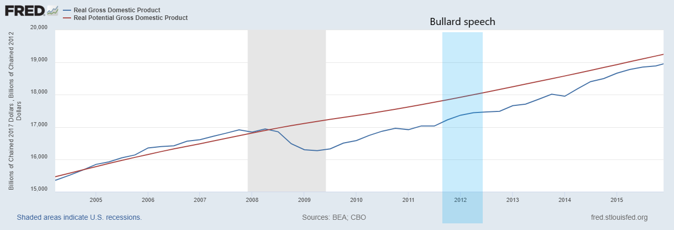
The Output-gap According to the FRB ... St. Louis

The FRB of St. Louis publishes "oficial" US data for Real GDP and Potential GDP.

The Natural Rate of Unemployment (NRU)

4. Readings

Point 1

• For this point, there is no compulsory reading.

• However, Dirk Krueger (2007). "Quantitative Macroeconomics: An Introduction" (Chapter 2), manuscript, Department of Economics University of Pennsylvania, is well suited for the material covered here.

• This text is a small one (12 pages), easy to read, and beneficial for studying the stylized facts of business cycles, mainly to understand how the Hodrick-Prescott filter is calculated. However, notice that, as mentioned, it is not compulsory reading.

Point 2

• For this point, there is no compulsory reading. However, any modern textbook on time series will cover this subject.
• At an introductory level, see sections 11.8 and 11.9 of the textbook: Diebold, F. X. (1998). Elements of forecasting. South-Western College Pub, Cincinnati.
• At a more advanced level, see, e.g., section 2.3.2 of the textbook: Lütkepohl, H. (2007). New introduction to multiple time series analysis (2nd ed.), Springer, Berlin.

Point 3

• No textbook covers the topics/controversies mentioned in this section.
• This coursework intends to provide a framework for a better understanding of these controversies at the end of the course.
• All we have to handle is:
  • A little bit of mathematics
  • A little bit of computation
  • A little bit of macroeconomics